Marker-gene-guided dimensionality reduction (GDR)

GDR: marker Gene-guided Dimensionality Reduction

import piaso

piaso.settings.set_figure_params(style="cell")

set_figure_params sets the figure size, the font and the rest of the house style in one call, so the rcParams block that used to be here is no longer needed. cosg is not imported: nothing on this page calls it.

Load the data

We will be using a Multiome RNA dataset obtained from cortex at P57.

adata = piaso.data.load_dataset("adult_cortex_multiome_rna")
adata

adata.X=adata.layers['log1p'].copy()

INFOG normalization

INFOG normalises from the raw counts, so it takes layer='raw' rather than the log1p values in .X. It takes under two seconds here.

piaso.tl.infog(adata,
               layer='raw',
               n_top_genes=3000,)

Visualize with PCA-based UMAP

First, we will use a standard PCA-based UMAP to visualize the batches and cell types in the dataset. This helps in assessing the presence of batch effects.

piaso.tl.neighbors(adata, use_rep='X_pca', n_neighbors=15, random_state=10)
piaso.tl.umap(adata, use_rep='X_pca')

piaso.pl.embedding(adata,
                   color=['Sample', 'CellTypes'],
                   basis='X_umap',
                   palette=piaso.pl.color.d_color4,
                   ncols=1)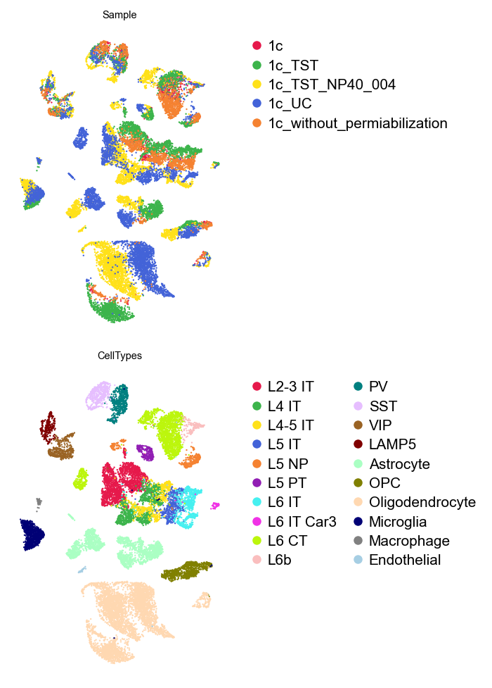

The UMAP plot clearly shows batch effects in the dataset.

Dimensionality reduction with GDRParallel

In this turorial we will show how GDR works when only batch information is available and clusters or cell type informations isn’t available. In this case, runGDR clusters the data and infers the groups.

piaso.tl.runGDRParallel(adata,
                        batch_key='Sample',
                        groupby=None,
                        n_gene=20,
                        mu=10,
                        resolution=3.0,
                        layer='infog',
                        infog_layer='raw',
                        score_layer='infog',
                        scoring_method='piaso',
                        use_highly_variable=True,
                        n_highly_variable_genes=5000,
                        n_svd_dims=50,
                        key_added='X_gdr',
                        max_workers=32,
                        calculate_score_multiBatch=False,
                        verbosity=0)

29 seconds on 17,412 cells. X_gdr comes out with 161 dimensions — one per marker-gene group GDR found across the five batches, not a number you chose.

Visualize GDR results with UMAPs

piaso.tl.neighbors(adata, use_rep='X_gdr', n_neighbors=15, random_state=10)
piaso.tl.umap(adata, use_rep='X_gdr')

piaso.pl.embedding(adata,
                   color=['Sample', 'CellTypes'],
                   basis='X_umap',
                   palette=piaso.pl.color.d_color4,
                   ncols=1)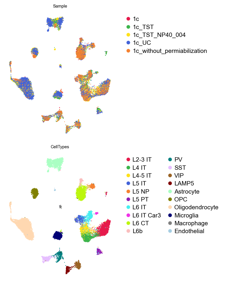

GDR effectively integrates batches and separates cell types using only dimensionality reduction, without additional integration methods.

What the two pictures are worth, as a number

The figures above are the usual evidence for an integration claim, and they are easy to over-read. So measure it: for each cell take its 30 nearest neighbours in the embedding and ask what fraction come from a different batch, and what fraction share its cell type.

from sklearn.neighbors import NearestNeighbors

batch = adata.obs['Sample'].astype(str).values
ctype = adata.obs['CellTypes'].astype(str).values

for rep in ('X_pca', 'X_gdr'):
    ind = NearestNeighbors(n_neighbors=31).fit(
        adata.obsm[rep]).kneighbors(adata.obsm[rep])[1][:, 1:]
    print(rep,
          (batch[ind] != batch[:, None]).mean(),      # batch mixing
          (ctype[ind] == ctype[:, None]).mean())      # cell-type purity

	batch mixing	cell-type purity
perfectly mixed would give	0.755	—
X_pca	0.186	0.966
X_gdr	0.529	0.957

GDR nearly triples batch mixing — 0.186 to 0.529 against a ceiling of 0.755 — and gives up 0.9 percentage points of cell-type purity to do it. That is the trade the pictures show, stated as a number: most of the batch structure is gone, and essentially none of the cell-type structure is.

Note the ceiling. If the embedding were perfectly mixed, a cell’s neighbours would look like the dataset as a whole, and with these five unequal samples that is 0.755, not 1.0. Comparing 0.529 against 1.0 would understate the result; against 0.755 it is about 70% of the way to complete mixing.

Do not use silhouette for this

Silhouette is the obvious metric and the wrong one here. X_pca has 50 dimensions and X_gdr has 161 — one per marker-gene group — and silhouette moves with dimensionality, so it scores GDR worse on both counts while the figures plainly show the opposite. The k-nearest-neighbour fractions above only use the ordering of distances, so they are comparable between spaces of different width.

groupby: unsupervised, or guided by labels you already have

groupby decides where the marker genes come from, and it is the parameter worth understanding before any other.

groupby=None (unsupervised). GDR clusters each batch on its own, calls markers for those de novo clusters with COSG, and builds the embedding from them. Nothing outside the expression matrix is used, so this is the setting for a dataset you have not annotated yet, and the one to use when the embedding will be the basis for annotation. It is also the honest setting for a benchmark: an embedding built from labels cannot then be judged on how well it separates those labels.

piaso.tl.runGDR(adata, batch_key='Sample', groupby=None,
                n_gene=20, layer='infog', key_added='X_gdr')

groupby='CellTypes' (guided). When you already trust an annotation, GDR calls markers for those cell types instead of for de novo clusters. The embedding is then organised around the distinctions you care about rather than around whichever clusters the resolution happened to produce. This is the setting for a reference atlas you will project new data into, for a figure where the annotation is settled, and for the case where a rare population is biologically important but too small for de novo clustering to separate.

piaso.tl.runGDR(adata, batch_key='Sample', groupby='CellTypes',
                n_gene=20, layer='infog', key_added='X_gdr_supervised')

Which to use:

	groupby=None	groupby='CellTypes'
marker genes from	de novo clusters, per batch	your labels
use when	the data is unannotated, or the embedding will be used to annotate it	the annotation is settled and you want the embedding organised around it
rare populations	may be merged into a neighbouring cluster before markers are called	kept, because the label keeps them
for benchmarking	yes	no: the labels are in the embedding, so scoring the embedding on those labels is circular

Both take batch_key. With groupby=None markers are called per batch and then pooled, which is what makes the embedding batch-aware without a separate integration step.

A worked comparison of the two settings — on a differentiation trajectory, where groupby="clusters" gives 8 groups and groupby=None finds 18 — is in GDR on developmental data. It is also the page that explains why the lower silhouette there is not the worse embedding.

Where to go next

Once the embedding exists, the rest of the ecosystem runs on it:

Cell type prediction with GDR	Transfer labels from an annotated reference through this embedding.
projectGDR	Freeze a reference’s GDR space and project new data into it, without re-fitting.
GDR on developmental data	The groupby comparison above, worked through on stages rather than terminal cell types.
GDR and SVD on 1.5 million cells	Both embeddings over one atlas: runtime, peak memory, and what each separates.
GDR at scale	200,000 cells streamed from a cytome.
GDR on spatial data	Eight embryo stages in one embedding.
GDR on scATAC-seq	The same idea on accessibility rather than expression.
GDR beyond transcriptomics	Images as expression matrices — what GDR separates on data that is not single-cell at all.

And two that use a GDR embedding without being about GDR:

• COSG markers — marker genes for the clusters you find here, with significance.
• Marker-based cell type prediction — annotation from a marker database, smoothed over neighbours in this space.