Local Leiden clustering
Finer clustering on selected cluster(s)
The leiden_local in PIASO is different from using the restrict_to parameter in scanpy’s tl.leiden function, which is running the clustering based on the cell similarity graph built from the whole gene expression matrix containing all the cells. PIASO’s leiden_local function will rerun the dimensional reduction for the selected cluster(s) first and then run the clustering on these cells, so as to better capture the heterogeneity in selected cells.
import pandas as pdimport scanpy as scimport osfrom matplotlib import cmimport loggingfrom matplotlib import rcParams
# To modify the default figure size, use rcParams.piaso.settings.set_figure_params(style="cell")rcParams['figure.figsize'] = 5, 5rcParams['font.sans-serif'] = "Arial"rcParams['font.family'] = "Arial"sc.settings.verbosity = 3sc.logging.print_header()
import piasoLoad the data
We will use the 20k subsampled version of the Seattle Alzheimer’s Disease Brain Cell Atlas (SEA-AD) project dataset described in detail in Gabitto et. al. (2024). We will be using the scRNA-seq data from the dataset in this tutorial. Please refer to the Introduction tutorial to learn more about how it was preprocessed and normalized.
Download the subsampled, pre-processed dataset from Google Drive: https://drive.google.com/file/d/1pDBIgPvEO-sBuIMEhrvVhnf7tfU7H6Xy/view?usp=drive_link
The original data is available on https://portal.brain-map.org/explore/seattle-alzheimers-disease
# Download from Google Drive:# https://drive.google.com/file/d/1pDBIgPvEO-sBuIMEhrvVhnf7tfU7H6Xy/viewdata_dir = "." # Update to your download directoryadata = sc.read(data_dir + '/SEA-AD_RNA_MTG_subsample_excludeReference_20k_piaso_preprocessed.h5ad')adataVisualize with UMAP
sc.pl.umap(adata, color=['Subclass'], palette=piaso.pl.color.d_color4, ncols=1, size=10, frameon=True)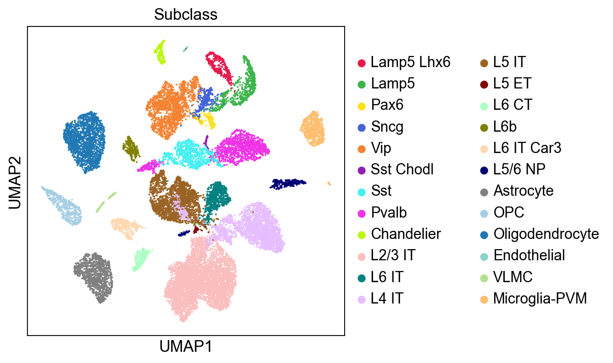
Cluster the data with Leiden algorithm
%%timesc.tl.leiden(adata,resolution=0.5,key_added='Leiden',flavor="igraph",n_iterations=-1)logging.getLogger('matplotlib.font_manager').disabled = Truesc.pl.umap(adata, color=['Leiden'], palette=piaso.pl.color.d_color4, legend_fontsize=12, legend_fontoutline=2, legend_loc='on data', ncols=1, size=10, frameon=False)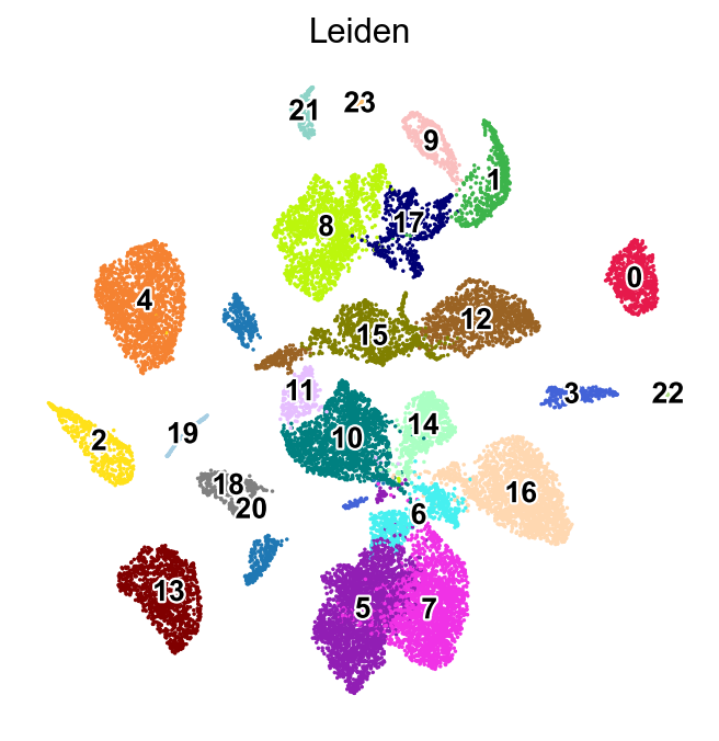
Run leiden_local on one cluster
Here, we run leiden_local on cluster 8 from the leiden clustering.
piaso.tl.leiden_local(adata, clustering_type='each', groupby='Leiden', groups=['8'], resolution=0.2, batch_key=None, key_added='Leiden_local_one', dr_method='X_svd_full', copy=False)sc.pl.umap(adata, color=['Leiden'], groups=['8'], palette=piaso.pl.color.d_color4, legend_fontsize=12, legend_fontoutline=2, legend_loc='on data', ncols=1, size=10, frameon=False)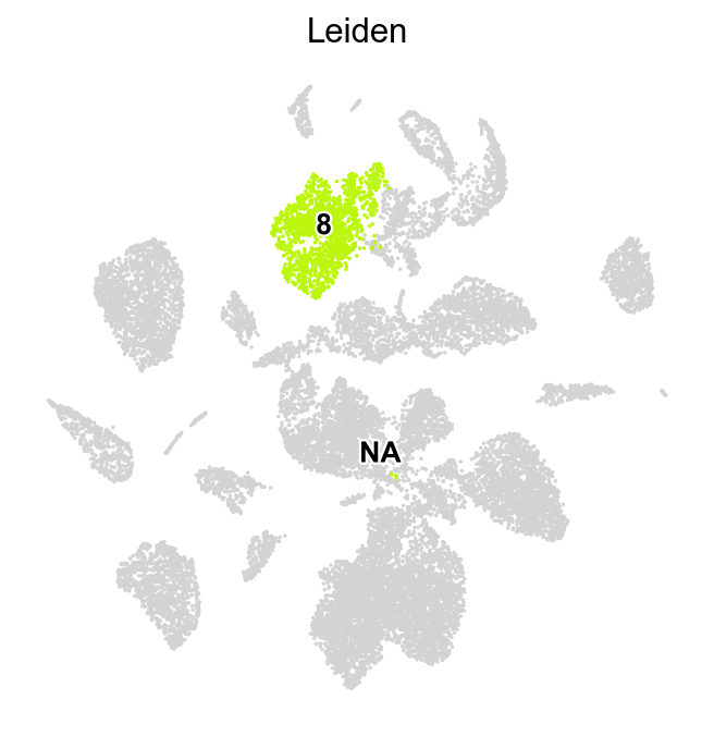
sc.pl.umap(adata, color=['Leiden_local_one'], groups=['8-0','8-1','8-2','8-3'], palette=piaso.pl.color.d_color4, legend_fontsize=12, legend_fontoutline=2, ncols=1, size=10, frameon=False)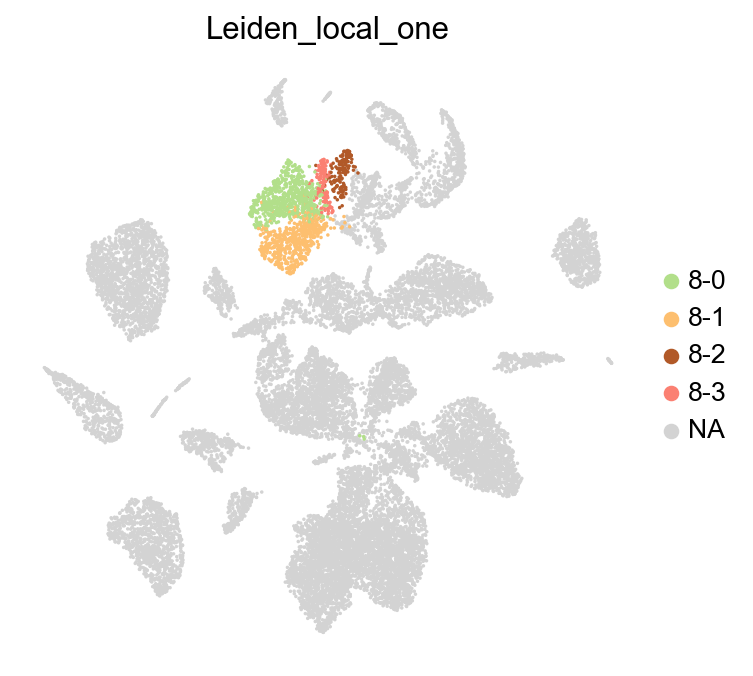
Identify markger genes in subclusters
Identify the marker genes for each sub-cluster identified by leiden local along with all the leiden clusters.
import cosgn_gene=30cosg.cosg(adata, key_added='cosg', use_raw=False, layer='log1p', ## e.g., if you want to use the log1p layer in adata mu=100, expressed_pct=0.1, remove_lowly_expressed=True, n_genes_user=100, groupby='Leiden_local_one')sc.tl.dendrogram(adata,groupby='Leiden_local_one',use_rep='X_svd')df_tmp=pd.DataFrame(adata.uns['cosg']['names'][:3,]).Tdf_tmp=df_tmp.reindex(adata.uns['dendrogram_'+'Leiden_local_one']['categories_ordered'])marker_genes_list={idx: list(row.values) for idx, row in df_tmp.iterrows()}marker_genes_list = {k: v for k, v in marker_genes_list.items() if not any(isinstance(x, float) for x in v)}
sc.pl.dotplot(adata, marker_genes_list, groupby='Leiden_local_one', layer='log1p', dendrogram=True, swap_axes=False, standard_scale='var', cmap='Spectral_r')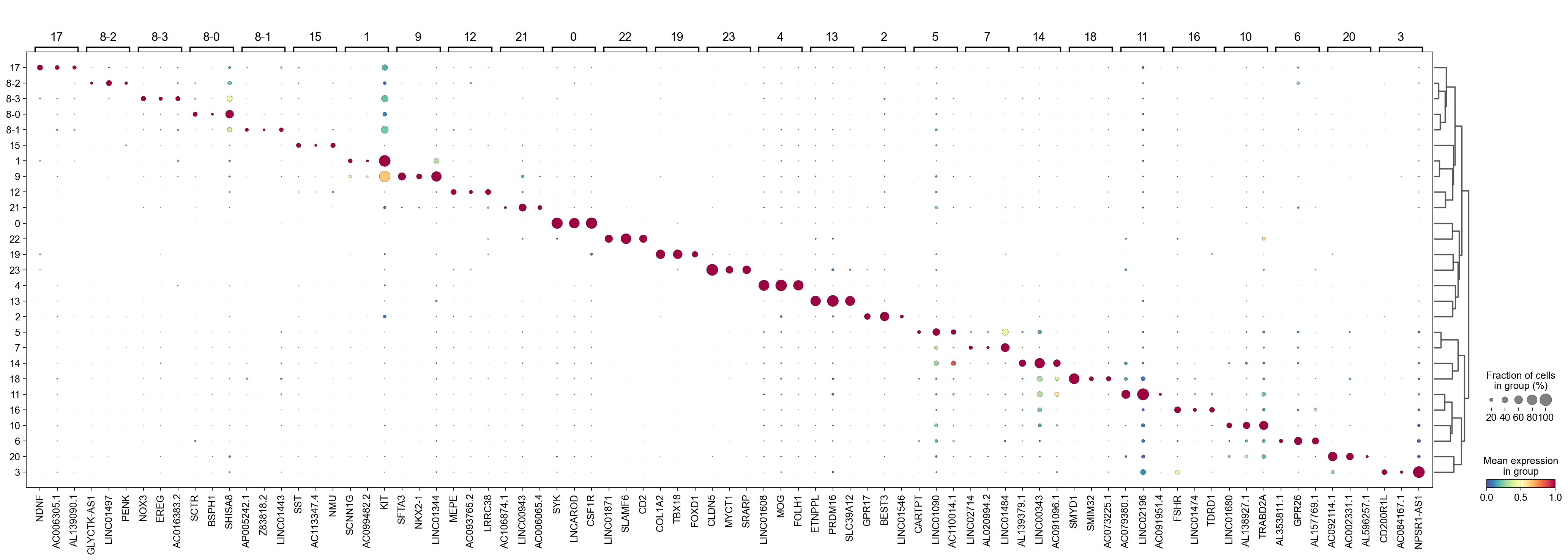
The dotplot reveals that the subclusters identified by leiden_local within leiden cluster 8 exhibit distinct marker genes, suggesting they may differ in nature. Our function successfully detects these differences and can differentiate between the subclusters.
Run leiden_local on multiple clusters
leiden_local can be run on multiple clusters together, either to identify subclusters within each distinct cluster or identify subclusters across all the given clusters.
Perform clustering independently within each group
piaso.tl.leiden_local(adata, clustering_type='each', groupby='Leiden', groups=['1','8','9','17'], resolution=0.2, batch_key=None, key_added='Leiden_local_many_each', dr_method='X_svd_full', copy=False)sc.pl.umap(adata, color=['Leiden_local_many_each'], groups=['1-0','1-1','8-0','8-1','8-2','8-3','9-0','9-1','17-0','17-1','17-2'], palette=piaso.pl.color.d_color4, legend_fontsize=12, legend_fontoutline=2, ncols=1, size=10, frameon=False)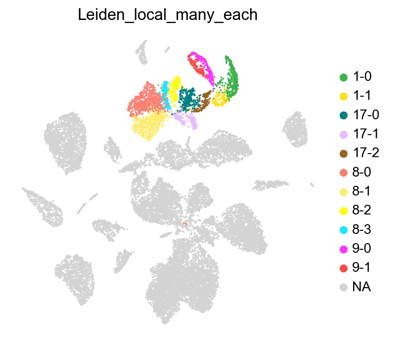
Perform clustering across all selected groups
Here, we will use leiden_local to identify sub-clusters across a group clusters. Let us select a group of subclasses from the data: Lamp5 Lhx6, Lamp5, Pax6, Sncg, and Vip, which are made of clusters ‘1’, ‘8’, ‘9’, and ‘17’.
piaso.tl.leiden_local(adata, clustering_type='all', groupby='Leiden', groups=['1','8','9','17'], resolution=0.5, batch_key=None, key_added='Leiden_local_many_all', dr_method='X_svd_full', copy=False)sc.pl.umap(adata, color=['Leiden_local_many_all'], groups=['M-0','M-1','M-2','M-3','M-4','M-5','M-6','M-7','M-8'], palette=piaso.pl.color.d_color4, legend_fontsize=12, legend_fontoutline=2, ncols=1, size=10, frameon=False)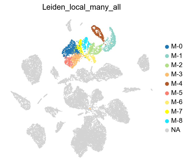
We can compare the subclusters identified by leiden_local with the annotated subclasses from the data, and observe that the identified clusters closely align with the actual subclasses.
sc.pl.umap(adata, color=['Subclass'], palette=piaso.pl.color.d_color4, ncols=1, size=10, frameon=True)