
KEGG and drug-target gene sets
PIASOscore covers the method. This page is the application: score two public databases across 20,000 human cortical nuclei, then hand the score matrix to COSG and ask which cell type each pathway — and each drug — belongs to.
import numpy as npimport pandas as pdimport anndata as adimport piaso, cosgimport gseapy as gp
piaso.settings.set_figure_params(style="cell")
adata = piaso.data.load_dataset("sea_ad_mtg_20k")piaso.tl.infog(adata, layer="UMIs", n_top_genes=3000) # .X is normalized here1. Two databases
gseapy fetches gene set libraries by name, so nothing needs downloading by
hand:
kegg = gp.parser.get_library("KEGG_2021_Human")drugs = gp.parser.get_library("DGIdb_Drug_Targets_2024")drugs = {k: v for k, v in drugs.items() if len(v) >= 5}len(kegg), len(drugs)(320, 659)The drug library is the interesting one: each set is the targets of one drug. Scoring it asks “which cell type expresses what this compound binds”, which is the first question in any repurposing or off-target discussion.
Dropping sets below five genes is not cosmetic: a two-gene set gives a score dominated by two genes’ noise, and there are hundreds of them.
2. Score both
def score_frame(sets):    matrix, names, _ = piaso.tl.score(adata, gene_list=sets)    a = ad.AnnData(X=np.asarray(matrix), obs=adata.obs.copy(),                   var=pd.DataFrame(index=list(names)))    a.obsm = adata.obsm.copy()    return a
kegg_scores = score_frame(kegg)     # 320 sets x 20,000 cells — 49.4 sdrug_scores = score_frame(drugs)    # 659 sets x 20,000 cells — 19.1 s
The drug library scores in less than half the time for twice as many sets, because its sets are small: cost tracks total genes, not set count.
3. Which pathway belongs to which cell type
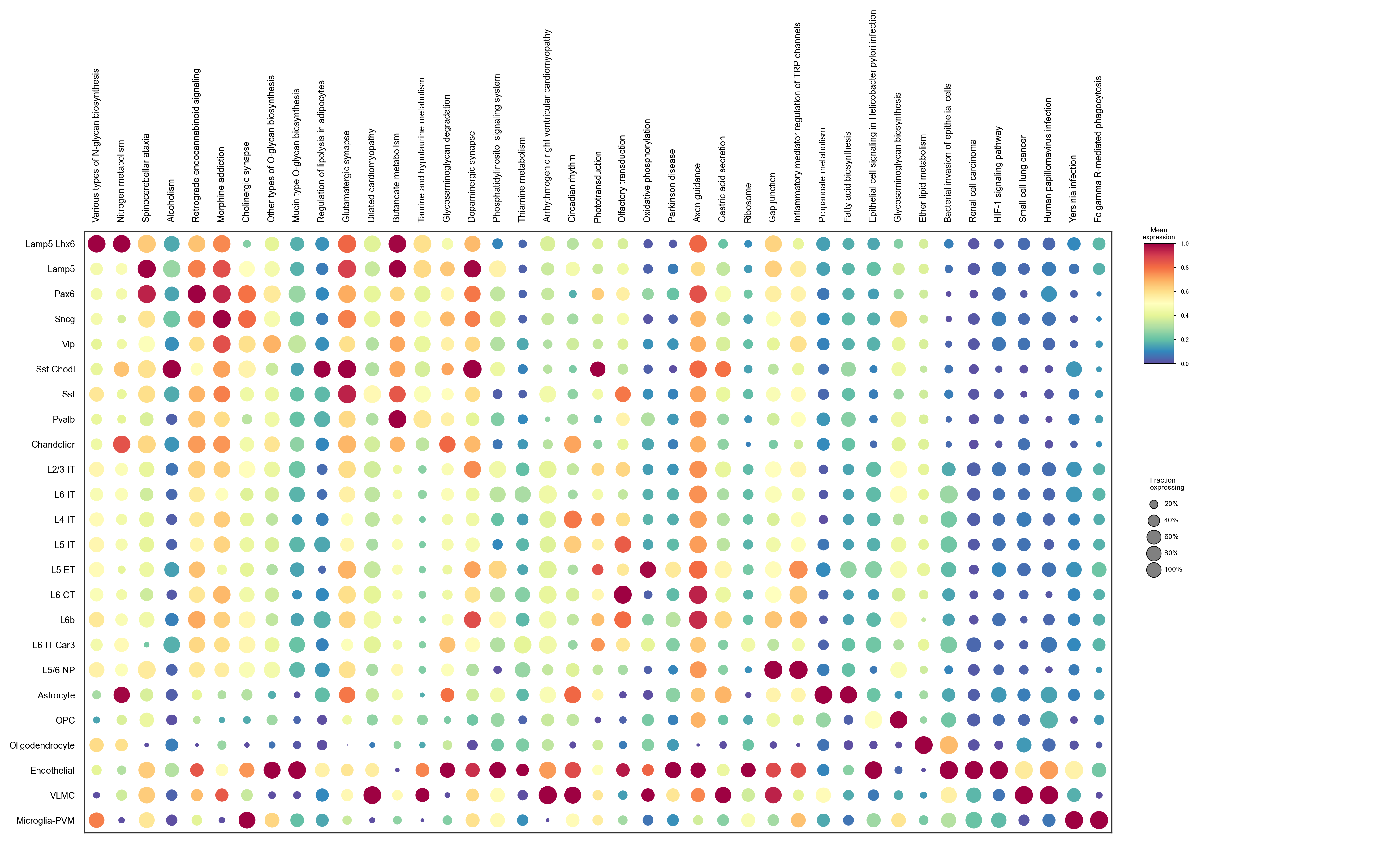
The score matrix is cells × sets, the same shape as cells × genes, so COSG works on it unchanged:
cosg.cosg(kegg_scores, key_added="cosg", groupby="Subclass", n_genes_user=5, mu=1, remove_lowly_expressed=False)pd.DataFrame(kegg_scores.uns["cosg"]["names"]).head(3)| subclass | top KEGG sets |
|---|---|
| Microglia-PVM | Yersinia infection; Fc gamma R-mediated phagocytosis; NOD-like receptor signaling |
| Oligodendrocyte | Ether lipid metabolism; Bacterial invasion of epithelial cells; AMPK signaling |
| Astrocyte | Propanoate metabolism; Fatty acid biosynthesis; PPAR signaling |
| Endothelial | Renal cell carcinoma; HIF-1 signaling; Hepatitis C |
| L2/3 IT | Dopaminergic synapse; Phosphatidylinositol signaling; Amphetamine addiction |
| Pvalb | Butanoate metabolism; Taurine and hypotaurine metabolism; Thermogenesis |
Read KEGG’s names, not KEGG’s titles. “Yersinia infection” and “Bacterial invasion of epithelial cells” are phagocytosis and cytoskeletal-remodelling gene sets curated from infection studies; “Renal cell carcinoma” and “Hepatitis C” are largely growth-factor and interferon signalling. Nothing here is a claim about bacteria or cancer in this tissue.
Translated: microglia score on phagocytosis and innate immunity; oligodendrocytes on lipid metabolism, which is myelin; astrocytes on fatty-acid synthesis; endothelium on hypoxia signalling; excitatory neurons on synaptic transmission. Every one is correct, and none was supplied.
4. Which drug targets which cell type
Same call, different library:
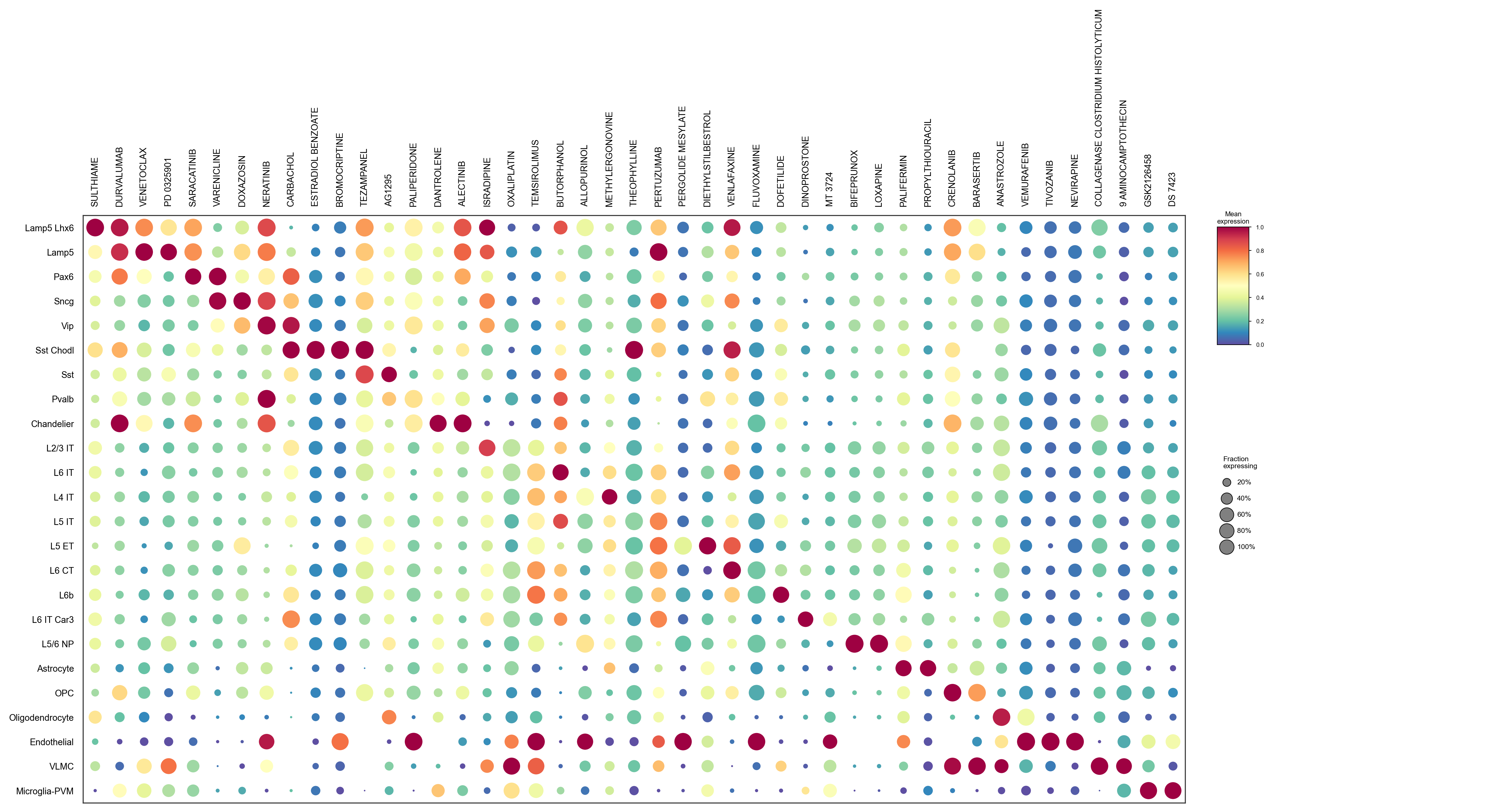
| subclass | top drugs by target-set score |
|---|---|
| VLMC | COLLAGENASE CLOSTRIDIUM HISTOLYTICUM; 9-aminocamptothecin; dacarbazine |
| Endothelial | TIVOZANIB; nevirapine; MGCD265 |
| Microglia-PVM | GSK2126458; DS-7423; XL147 |
| Astrocyte | palifermin; propylthiouracil; MK-2461 |
| L2/3 IT | isradipine; oxaliplatin; mosapride |
Two of these are hard checks that the method is not producing noise:
- VLMC’s top drug is a collagenase. Its “targets” are collagens, and VLMC — vascular leptomeningeal cells — are the collagen-producing cells of the meninges. The SCALAR page reaches the same conclusion from a completely different direction, finding COL1A2 and COL6A2 signalling from VLMC as the strongest interactions in the dataset.
- Endothelium’s top drugs are TIVOZANIB and MGCD265, both receptor tyrosine kinase inhibitors targeting VEGFR — the endothelial receptor family.
The three microglial hits (GSK2126458, DS-7423, XL147) are all PI3K inhibitors, which is consistent but less specific: PI3K is expressed widely.
5. One drug at a time
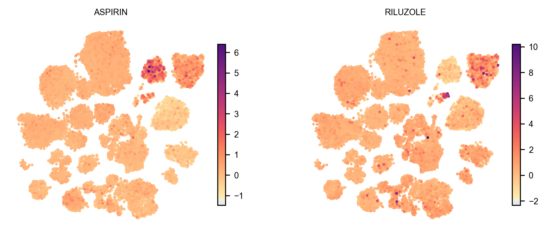
for drug in ["ASPIRIN", "RILUZOLE"]: by = (drug_scores.obs .assign(v=np.asarray(drug_scores[:, drug].X).ravel()) .groupby("Subclass", observed=True)["v"].median() .sort_values(ascending=False)) print(drug, by.head(3).to_dict())for d in ["ASPIRIN", "RILUZOLE"]: v = np.asarray(drug_scores[:, d].X).ravel() lo, hi = np.percentile(v, [2, 98]) # a few cells own the raw range piaso.pl.plotEmbedding(drug_scores, basis="X_umap", color=d, cmap="Spectral_r", vmin=lo, vmax=hi)ASPIRIN Microglia-PVM 0.445 | VLMC 0.182 | L6 IT Car3 0.175RILUZOLE Chandelier 0.363 | Sncg 0.254 | Sst Chodl 0.243Aspirin’s targets are the cyclooxygenases, and microglia are the prostaglandin producers of the brain: a factor of 2.4 above the next subclass. Riluzole’s targets are sodium channels and glutamate handling, and its top three are all inhibitory interneuron types.
What this is and is not
- Is: a per-cell readout of where a pathway or a compound’s targets are expressed, with the depth confounding removed by the control sets.
- Is not: an efficacy prediction. Target expression is necessary, not sufficient: it says nothing about whether the drug reaches the tissue, or what the consequence of binding is.
- Target annotations are incomplete and biased toward well-studied compounds. A drug scoring low may simply have few curated targets.
6. ChEMBL: binding affinities, not just a target list
The gseapy library above gives a list of targets. ChEMBL gives the measured
activities behind them, which lets the gene sets be built to a stated potency
rather than taken as given. piaso.data fetches the table and does the
filtering:
targets = piaso.data.load_chembl_targets() # fetches ~2.7 GB on first uselen(targets)This is opt-in and large. The merged ChEMBL 30 table is 2.7 GB on disk and wants roughly 10 GB of RAM to read; nothing downloads it implicitly. If you only need a target list, stay with the gseapy libraries in §1.
What the filter is doing
Raw ChEMBL is every measured activity, including inactive ones, assays of the wrong kind, and compounds that never left preclinical. Six steps turn it into gene sets, and the defaults are visible rather than buried:
from piaso.data import filter_chembl_activities, PCHEMBL_THRESHOLDS
PCHEMBL_THRESHOLDS
{'none': 6.0, # 1 uM -- unclassified 'NHR': 7.0, # 100 nM -- nuclear hormone receptors 'GPCR': 7.0, # 100 nM 'Ion Channel': 5.0, # 10 uM 'Kinase': 7.53} # 30 nMpChEMBL is −log10(activity), so larger is tighter. The threshold has to depend on the target class: 30 nM is unremarkable for a kinase inhibitor and exceptional for an ion-channel blocker, so a single global cut-off would keep the wrong compounds for half the classes. Two activities with the same pChEMBL of 6.5 get opposite verdicts: kept for an ion channel, dropped for a kinase.
targets = piaso.data.load_chembl_targets( drug_max_phase=4, # approved drugs only assay_type="F", # functional: measures a biological effect add_drug_mechanism=True, # a curated mechanism outranks any assay remove_inactive=True, include_active=True,)Two of those arguments do not remove anything. add_drug_mechanism and
include_active mark rows as protected so the later filters cannot drop
them. A compound with a curated mechanism of action survives an assay-type or
potency cut it would otherwise fail, because a curated mechanism is better
evidence than any single measurement.
That is not a small correction. On ChEMBL 30 the call above keeps 39,660 of
6,708,016 activities and yields 2,447 drugs; with add_drug_mechanism=False
the same call keeps 12,930 and yields 827. Two thirds of the dictionary is
there because a curator recorded a mechanism, not because an assay row survived
the potency cut. Getting the argument backwards does not fail — it silently
returns a third of the drugs, which is why verbose=True (the default) prints
what each step removed:
max_phase in [4]: 6,708,016 -> 379,923 (6,328,093 removed) protected by drug mechanism: 28,188 assay_type in ['F']: 379,923 -> 77,683 (302,240 removed) inactive activity comments: 77,683 -> 68,372 (9,311 removed) protected by active comment: 9,753 pChEMBL threshold: 68,372 -> 39,660 (28,712 removed) kept 39,660 of 6,708,016 activities (0.59%)Read the big gene sets sceptically
The result spans 1,196 genes, with a median of 2 targets per drug, but the
distribution has a tail, and the tail is not biology. The genes that appear in
the most drug sets are TDP1 (459 of 2,447 drugs), LMNA (248), EHMT2
(212), BLM (99): counterscreen targets from large public high-throughput
panels, where a great many approved drugs were measured once and passed a
potency cut. LEVODOPA picks up sixteen targets this way, most of them DNA
repair enzymes.
The specific hits are fine — CHEMBL25|ASPIRIN gives PTGS1, PTGS2,
P2RY12; CHEMBL941|IMATINIB gives ABL1, KIT, PDGFRA, PDGFRB, LCK.
Scoring an unfamiliar drug set is worth a look at its members first, and a
promiscuous target scoring across every cell type in your data is a property of
the screen it came from, not of the tissue.
Then it is a gene set dictionary like any other:
# One set, passed as a list: key_added names the column. Wrapping it in a# dict makes it the many-sets call, where each score is named by its own key.piaso.tl.score(adata, gene_list=targets["CHEMBL25|ASPIRIN"], layer="infog", key_added="aspirin_targets")piaso.pl.embedding(adata, basis="X_umap", color="aspirin_targets", cmap="Spectral_r")drug2cell
This analysis is from Kanemaru et al. (Nature 2023), whose drug2cell package
introduced it. drug2cell is not required here. The part of it used to
build the dictionary is a sequence of pandas filters, reimplemented in
piaso.data so the gene sets can be built with pandas alone and the thresholds
are visible in the call rather than inside a package.
One deliberate difference: where drug2cell raises if the table contains a
target class absent from the threshold dict, load_chembl_targets falls back to
default_pchembl and reports which classes took the fallback. A vocabulary that
has drifted since the thresholds were written is not a reason to fail the whole
build.
What this page used to do
The v1.1.0 version used drug2cell with a ChEMBL table read from a hard-coded
local path, which made it unreproducible off the machine it was written on. The
gseapy route in §1–5 runs from a clean install with no downloads; §6 gives the
ChEMBL route back, fetched and filtered by PIASO. The original is preserved at
/tutorials/previous/kegg-chembl/.