GDR on developmental data

Most GDR examples group by terminal cell type. Development is the harder case: the groups are stages of one process, they grade into each other by construction, and an embedding that separates them cleanly is doing something a variance-driven one will not.

This uses pancreatic endocrinogenesis — eight stages from ductal progenitor through Ngn3-low and Ngn3-high to the four endocrine fates — and compares GDR against plain SVD on the same matrix.

3. Pancreatic endocrinogenesis: a trajectory, not clusters

Cell types are discrete. A differentiation trajectory is not, and it is the harder case for a method that builds its space from group-specific features.

p = ad.read_h5ad("endocrinogenesis_day15.h5ad")   # ~52 MB, direct download
p.layers["raw"] = p.X.copy()
p.obs["clusters"].value_counts()

Ductal           916
Ngn3 high EP     642
Pre-endocrine    592
Beta             591
Alpha            481
Ngn3 low EP      262
Epsilon          142
Delta             70

Ductal → Ngn3-low → Ngn3-high → pre-endocrine → the four hormone-producing fates. Neighbouring stages are genuinely continuous with each other.

piaso.tl.infog(p, layer="raw", n_top_genes=3000)
piaso.tl.runSVD(p, layer="infog", n_components=50, key_added="X_svd")
piaso.tl.neighbors(p, use_rep="X_svd", n_neighbors=15)
piaso.tl.umap(p, use_rep="X_svd")
piaso.pl.embedding(p, basis="X_umap", color="clusters")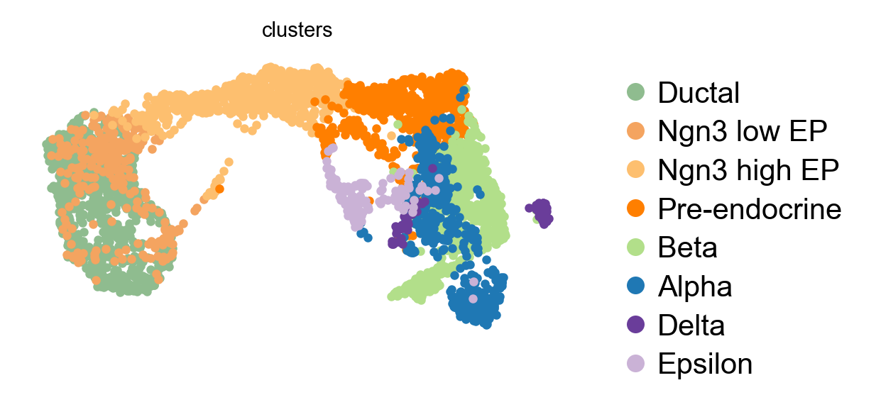

piaso.tl.runGDR(p, batch_key=None, groupby="clusters", n_gene=20, mu=10,
                layer="infog", score_layer="infog")
piaso.tl.neighbors(p, use_rep="X_gdr", n_neighbors=15)
piaso.tl.umap(p, use_rep="X_gdr", key_added="X_umap_gdr")
piaso.pl.embedding(p, basis="X_umap_gdr", color="clusters")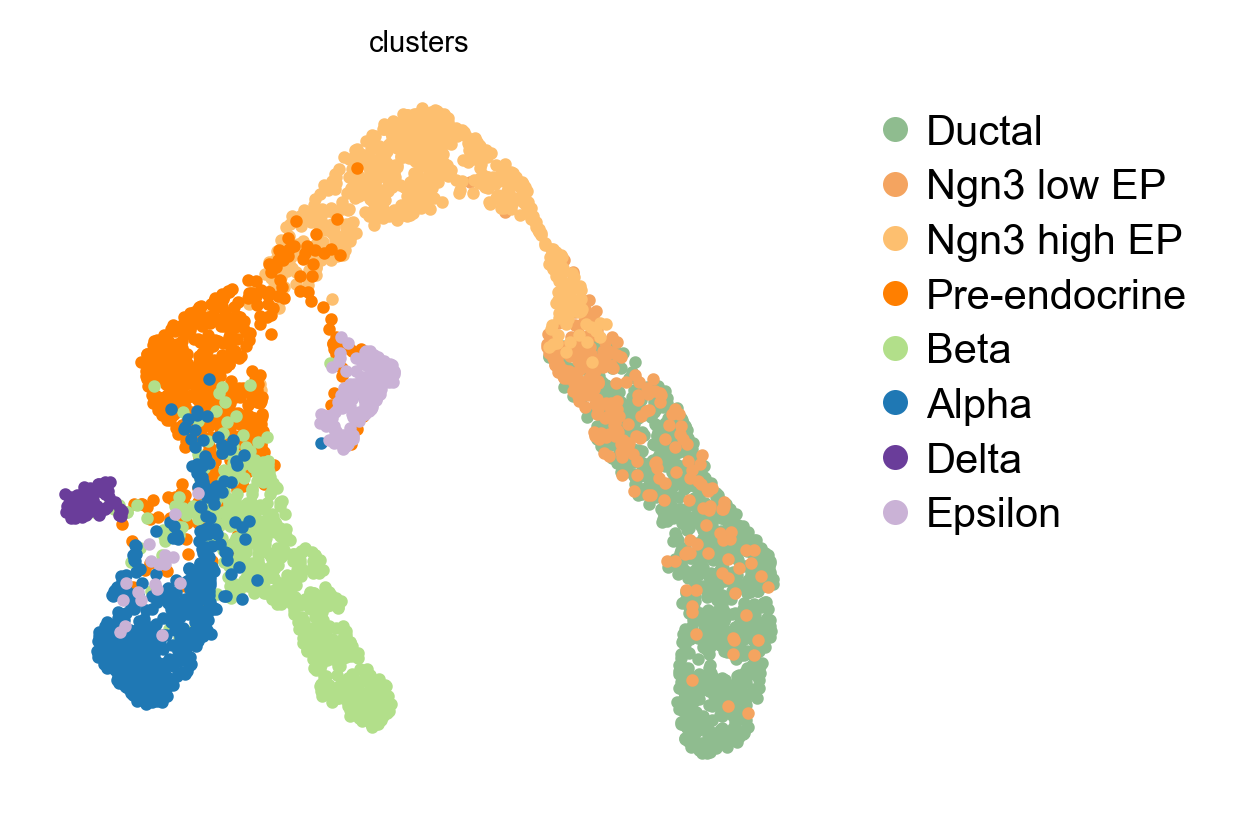

Supervised or not: what groupby decides

groupby names the grouping GDR builds its marker sets from. Passing a column uses your annotation; passing None makes GDR cluster the data itself first. On a trajectory that choice matters more than usual, because the annotation is a set of stage labels someone drew across a continuum.

# supervised: build markers from the eight annotated stages
piaso.tl.runGDR(p, batch_key=None, groupby="clusters", n_gene=20, mu=10.0,
                layer="infog", score_layer="infog")

# unsupervised: let GDR find its own groups first
piaso.tl.runGDR(p, batch_key=None, groupby=None, n_gene=20, mu=10.0,
                layer="infog", score_layer="infog")

n_gene=20 is the default; the earlier version of this page used 30, which is a reasonable choice but not the one you get by omitting the argument.

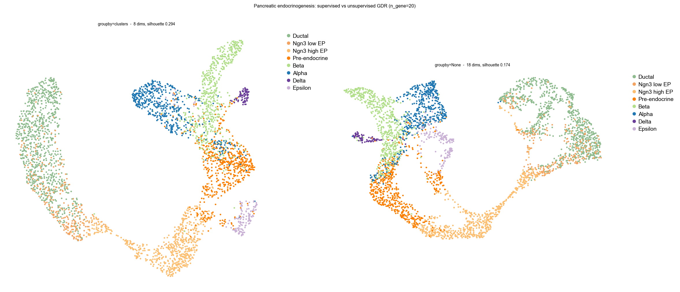
	dims	silhouette vs clusters
groupby="clusters"	8	0.294
groupby=None	18	0.174

The lower silhouette is not the worse embedding. Silhouette is measured against the eight annotated stages, and the supervised run built its axes from exactly those labels, so it is being scored on the thing it optimised. The unsupervised run found 18 groups where the annotation has 8 — and in the right panel that shows up as structure the labels do not carry: the Ductal arm separates into two lobes, and Epsilon pulls away from Pre-endocrine rather than sitting inside it.

So the rule is about what you trust. If the annotation is the object of study, groupby it and the embedding will organise around it. If the annotation is coarse — a stage label spanning a continuum, or a cell type you suspect contains substructure — groupby=None will find heterogeneity the labels average over, and the silhouette against those labels will drop while the embedding gets more informative, not less.

The trade, in two numbers

embedding	silhouette	15-NN accuracy
SVD	0.100	0.886
GDR	0.309	0.870

from sklearn.model_selection import train_test_split
from sklearn.neighbors import KNeighborsClassifier
from sklearn.metrics import silhouette_score

def knn_acc(X, y, seed=0):
    Xtr, Xte, ytr, yte = train_test_split(X, y, test_size=0.3,
                                          random_state=seed, stratify=y)
    return KNeighborsClassifier(15).fit(Xtr, ytr).score(Xte, yte)

y = p.obs["clusters"].astype(str).values
for key in ("X_svd", "X_gdr"):
    print(key, knn_acc(p.obsm[key], y),
          silhouette_score(p.obsm[key], y, sample_size=3000, random_state=0))

Three times the separation for a 1.6% accuracy cost. The two numbers disagree because they measure different things: GDR builds its axes from the genes that distinguish the stages, so the stages end up compact and ordered — that is the silhouette — and the price is the local variation kNN was using to interpolate between neighbours. On a trajectory that variation is mostly noise, which is why the cost here is small.

GDR is a structure method, not a classifier. On developmental data that is exactly what you want: the question is usually what is the order and where are the transitions, not what label does this cell get.

The same trade on data that is not single-cell at all — where the cost is much larger — is in GDR beyond transcriptomics.

Notes

• n_gene=20 per group sets how aggressive the compression is. Raising it recovers kNN accuracy and lowers separation.
• Grouping by stage rather than by terminal type is the whole point; passing groupby a terminal-fate column would collapse the trajectory.