Spatial: Xenium with tissue-image overlay

This tutorial runs 10x Genomics’ public Xenium human breast cancer dataset end to end: 167,780 segmented cells × 313 genes, clustered and drawn on the DAPI morphology image — with the image, the coordinates, and their spatial index all stored inside one .cytome file. Requires cytome >= 0.2.6 and piaso >= 1.2.2; reading the OME-TIFF morphology once needs tifffile + imagecodecs.

Two routes to the same file. This page builds an AnnData, clusters it, and converts the result. The other route imports the 10x matrix straight into a cytome and never holds it in memory — Xenium, cytome-native. Use this one when the analysis is scanpy-shaped; use that one when the section is large or is one of many.

1. Download (10x public data, ~660 MB total)

B=https://cf.10xgenomics.com/samples/xenium/1.0.1/Xenium_FFPE_Human_Breast_Cancer_Rep1/Xenium_FFPE_Human_Breast_Cancer_Rep1
curl -O ${B}_cell_feature_matrix.h5
curl -O ${B}_cells.csv.gz
curl -O ${B}_morphology_mip.ome.tif     # DAPI maximum-intensity projection

2. Cells, coordinates, clustering

Save the raw counts before you normalise. piaso.tl.infog writes its result to adata.layers["infog"] and leaves adata.X alone, so nothing here destroys the UMIs — but nothing guarantees they survive either. One sc.pp.normalize_total later, in this notebook or the next one, overwrites X in place and they are gone for good. The line costs a copy and buys back every count-based analysis: differential expression, pseudobulk, re-normalising with different parameters, and writing an .h5ad a collaborator can still use.

adata.layers["counts"] = adata.X.copy()          # the raw UMIs, kept
import numpy as np
import pandas as pd
import piaso

adata = piaso.pp.read_10x_h5("Xenium_FFPE_Human_Breast_Cancer_Rep1_cell_feature_matrix.h5")
adata.var_names_make_unique()

cells = pd.read_csv("Xenium_FFPE_Human_Breast_Cancer_Rep1_cells.csv.gz")
cells["cell_id"] = cells["cell_id"].astype(str)          # h5 obs_names are strings
cells = cells.set_index("cell_id").loc[adata.obs_names]
adata.obsm["spatial"] = cells[["x_centroid", "y_centroid"]].to_numpy()  # microns

adata = adata[np.asarray(adata.X.sum(1)).ravel() >= 10].copy()   # light QC

piaso.tl.infog(adata, n_top_genes=2000)
piaso.tl.runSVD(adata, layer="infog", n_components=30, key_added="X_svd")
piaso.tl.neighbors(adata, use_rep="X_svd", n_neighbors=15)
piaso.tl.leiden(adata, resolution=1.0)
piaso.settings.set_figure_params(style="cell")   # one house style across every figure

164,000 cells and 29 clusters in under a minute.

3. The morphology image, at overlay resolution

The OME-TIFF is pyramidal; one mid-pyramid level (~3,200 × 4,400 px) is plenty for overlays. The one number that must be right is the scale factor: Xenium coordinates are microns, the full-resolution image is 0.2125 µm/px, and the pyramid level is a further downsampling — so scalef = level_scale / 0.2125 converts a micron coordinate to a stored pixel.

import tifffile

with tifffile.TiffFile("Xenium_FFPE_Human_Breast_Cancer_Rep1_morphology_mip.ome.tif") as tf:
    level = next(i for i, l in enumerate(tf.series[0].levels)
                 if max(l.shape[:2]) <= 8000)
    img = tf.series[0].levels[level].asarray()
    full_w = tf.series[0].levels[0].shape[1]

scalef = (img.shape[1] / full_w) / 0.2125        # micron -> stored pixel
p99 = np.percentile(img, 99)                     # display-normalise to uint8
img8 = np.clip(img.astype(np.float32) / p99 * 255, 0, 255).astype(np.uint8)

4. One file: matrix + coordinates + index + image

import cytome

ds = cytome.from_anndata(adata, output="xenium_breast.cytome")
# from_anndata already stored obsm['spatial'] as the `spatial` embedding AND
# built the R*-tree coordinate index. Add the image:
ds.add_spatial_image("xenium_rep1", "morphology", img8,
                     scalefactors={"tissue_morphology_scalef": scalef,
                                   "spot_diameter_fullres": 10.0})

The array is stored losslessly (raw + zstd) inside the same SQLite file — this dataset lands at ~1.1 GB all-in, and the image travels with the data.

5. Clusters on the tissue

piaso.pl.plotEmbedding(ds, color="leiden", basis="spatial",
                       image=True, img_key="morphology",
                       point_size=0.3, alpha=0.7, legend_loc="right")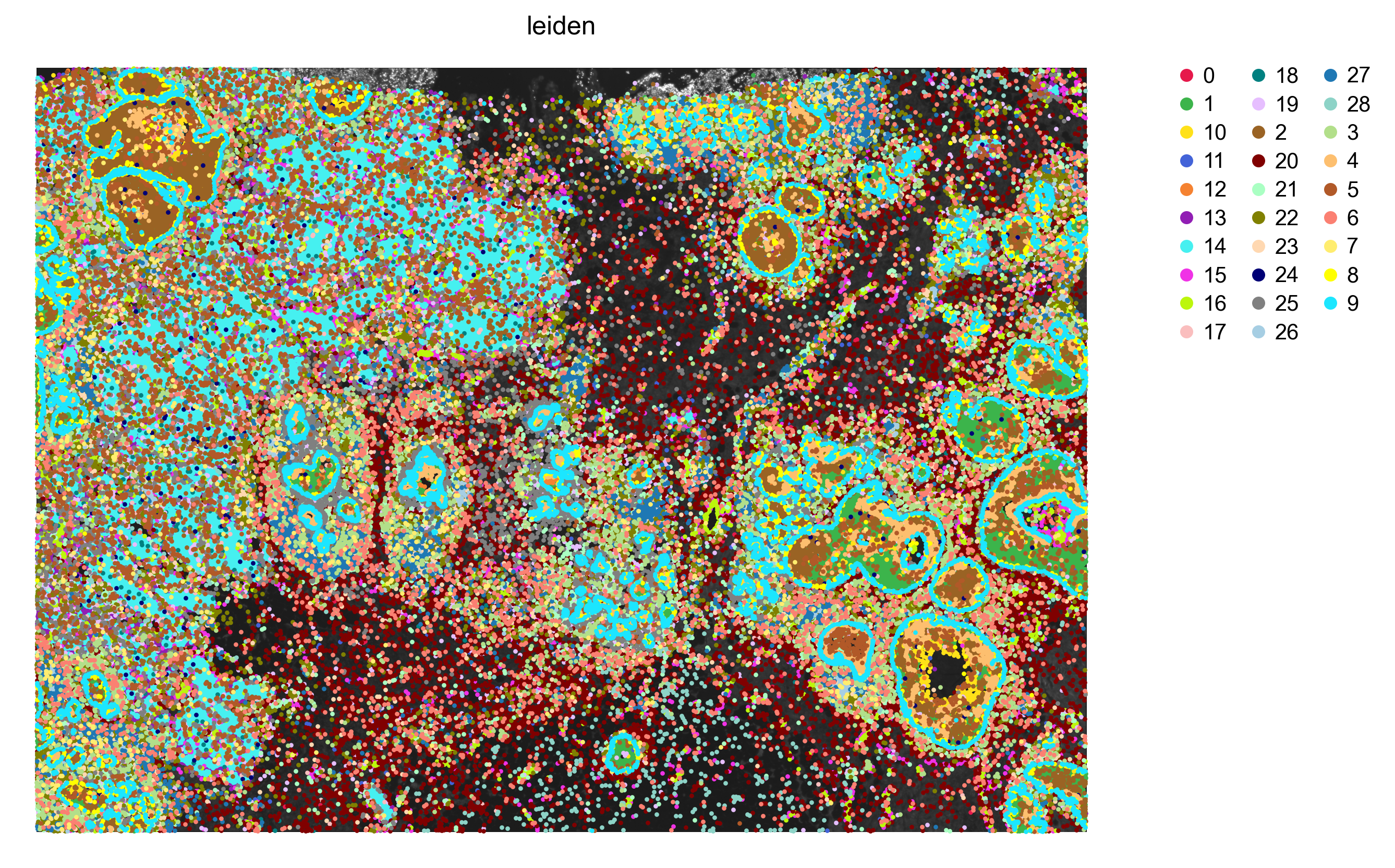

The cyan cluster traces the ductal boundaries — on a breast panel that is the myoepithelial signature, and having the DAPI behind the cells is what makes it readable. Orientation and units are handled for you: the image is drawn in coordinate space, so nothing needs flipping or scaling.

Per-cluster panels over the same tissue:

piaso.pl.plot_embeddings_split(ds, color="leiden", splitby="leiden",
                               basis="spatial", image=True,
                               img_key="morphology", ncol=5)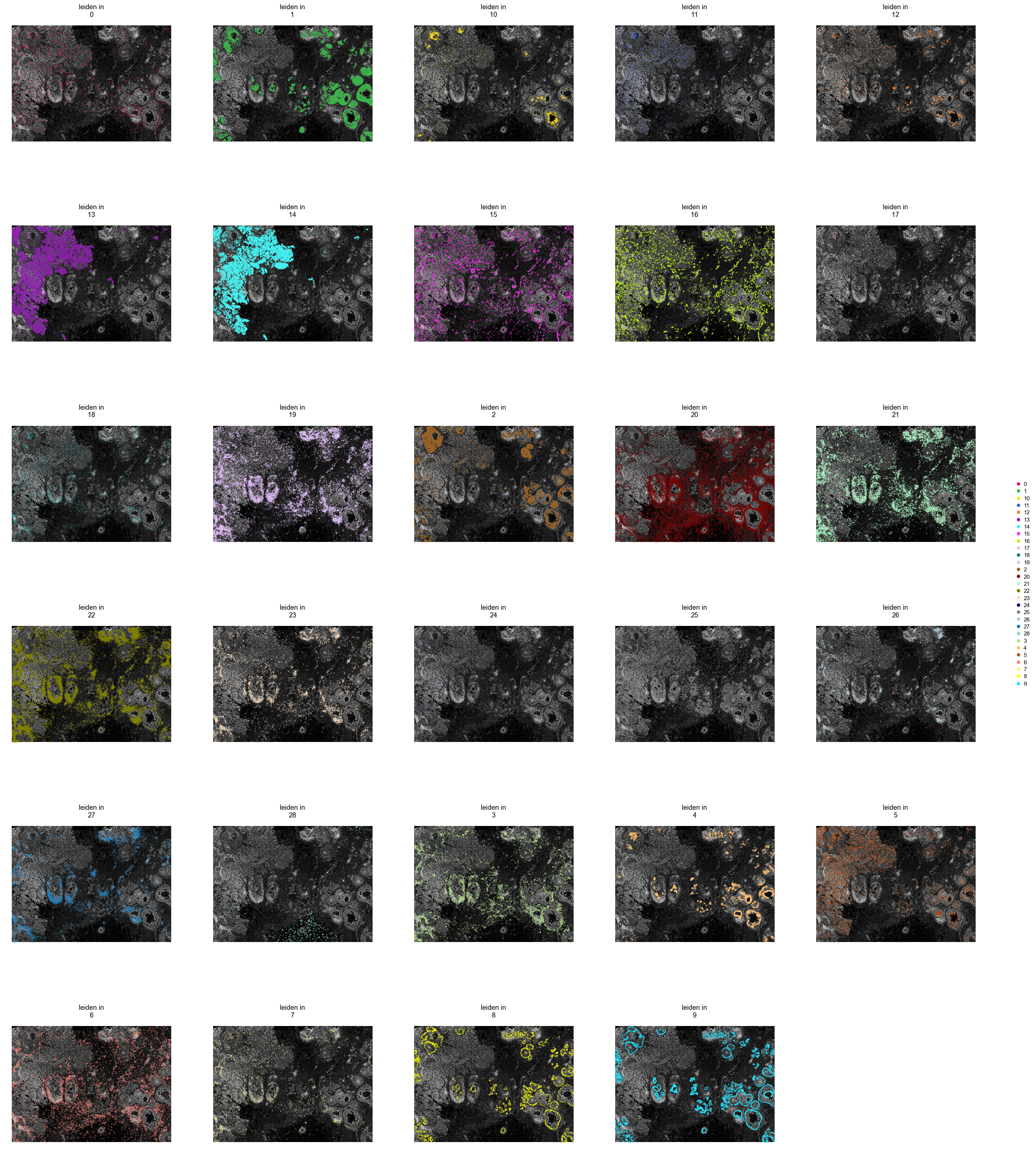

Twenty-nine panels, each one cluster over the same DAPI. This is the view that separates a cluster with a place from one without: ductal epithelium, stroma and immune infiltrate each occupy their own territory, while several clusters are scattered through the section and are telling you about state rather than location.

6. What the clusters are, and where one gene sits

Twenty-nine numbered clusters are not an answer. COSG names them from their own markers, and the same markers give a second embedding to check the first against.

import cosg

markers = cosg.cosg(ds, groupby="leiden", modality="RNA", layer="infog",
                    n_genes_user=5, mu=10, output_format="dict")

cosg.cosg on a cytome does not take key_added — there is no .uns to write to. It returns scores_dict keyed by (cluster, gene), plus groups_order and group_sizes; passing an AnnData-only keyword raises rather than being ignored, which is the behaviour you want when the two backends differ.

cluster	cells	top markers	what that is
9	6,308	KRT14, KRT5, MYLK	myoepithelium
1	13,087	CEACAM6, ESR1, AGR3	ER+ luminal tumour
13	12,359	TCIM, FOXA1, EPCAM	luminal epithelium
6	4,972	CD14, MRC1, CD163	macrophages
3	4,929	MZB1, TNFRSF17, SLAMF7	plasma cells
0	1,205	CPA3, CTSG, TPSAB1	mast cells

Cluster 9 is the cyan one from the overlay above: KRT14, KRT5 and MYLK are the myoepithelial layer, which is what “traces the ductal boundaries” means in gene terms rather than by eye.

The GDR embedding, from those markers

runGDR builds an embedding out of the genes that distinguish the clusters, so it answers a different question from SVD: not “what varies most” but “what separates these groups”.

piaso.tl.runGDR(ds, batch_key=None, groupby="leiden", n_gene=20, mu=10,
                layer="infog", score_layer="infog", key_added="X_gdr")

piaso.tl.neighbors(ds, use_rep="X_gdr", n_neighbors=15, key_added="gdr")
piaso.tl.umap(ds, use_rep="X_gdr", key_added="X_umap_gdr", neighbors_key="gdr")

piaso.pl.embedding(ds, basis="X_umap_gdr", color="leiden", ncol=1)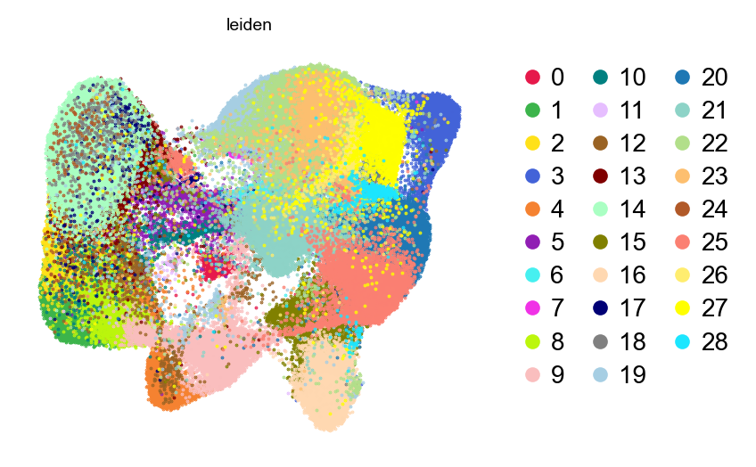

Xenium GDR embedding coloured by Leiden cluster

A 313-gene panel is already a marker-selected assay, so the two embeddings agree more than they would on whole-transcriptome data. What GDR adds here is separation between the epithelial clusters, which SVD leaves adjacent because they differ in a handful of genes against a shared background.

One gene, on the tissue

Everything that works for a cluster label works for a gene: the same call, the same image behind it.

piaso.pl.plotEmbedding(ds, color="KRT14", basis="spatial",
                       image=True, img_key="morphology",
                       point_size=0.3, alpha=0.7, cmap="Spectral_r")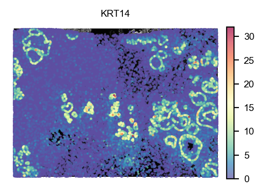

KRT14 expression over the morphology image

KRT14 draws the myoepithelial layer directly — a thin, continuous outline around each duct, with the luminal interior blank. That is the check the cluster overlay cannot give you on its own: the cluster is a label the algorithm assigned, while this is the measurement it was assigned from.

Colour comes from a feature rather than a cell column, so the default map is the continuous one; cmap= overrides it.

7. Regions of interest: cells and pixels from the same rectangle

cells_in_region is an indexed R*-tree lookup; spatial_images.crop cuts the matching pixels — both take the same coordinate ranges (microns here):

# Centre the window on the myoepithelial cluster from section 6, so the crop
# shows something the page has already named rather than an arbitrary square.
xy = ds.embeddings["RNA_spatial"]
leiden = ds.cells.to_pandas()["leiden"].astype(str).to_numpy()
cx, cy = xy[leiden == "9"].mean(axis=0)

roi_x, roi_y = (cx - 250, cx + 250), (cy - 250, cy + 250)   # a 500 um window

cells_in = ds.cells_in_region(x=roi_x, y=roi_y)

piaso.pl.plotEmbedding(ds, color="leiden", basis="spatial",
                       image=True, img_key="morphology",
                       cell_mask=cells_in,        # the R*-tree query, straight in
                       point_size=6, alpha=0.85, legend_loc="right")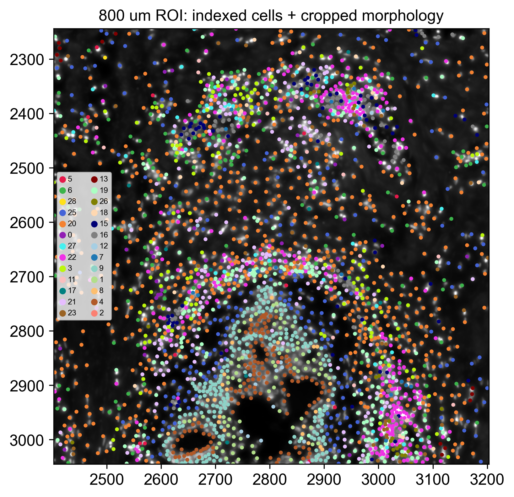

cells_in_region is the R*-tree query and cell_mask takes its result directly, so the region is chosen once and both the cells and the image follow it. image_crop (on by default) trims the morphology to the cells being drawn, which is why no extent arithmetic appears here: the alignment is the function’s job, not the caller’s.

The same call drew the whole slide in section 5. Only cell_mask and point_size changed — a region of interest is a view of the same figure, not a different one, and it is worth reaching for plotEmbedding rather than assembling axes by hand even when the hand-built version is short.