
COSG on spatial transcriptomics
Nothing about COSG is specific to dissociated cells. Any grouping of any observations works — and on spatial data the grouping is anatomical, which makes the result immediately checkable: plot the marker back in tissue space and see whether it lands on the organ it claims.
This page uses one E16.5 mouse embryo section from the MOSTA Stereo-seq atlas: 121,767 bins × 28,204 genes, with the paper’s 25 organ annotations.
1. The section
import cytome, cosg, piasoimport numpy as npimport pandas as pd
piaso.settings.set_figure_params()
ds = cytome.open("mosta_e16.cytome")ds.n_cells, pd.Series(np.asarray(ds.cells["annotation"])).nunique()
(121767, 25)piaso.pl.plotEmbedding(ds, color="annotation", basis="spatial", point_size=0.8, legend_loc="right", legend_ncol=2)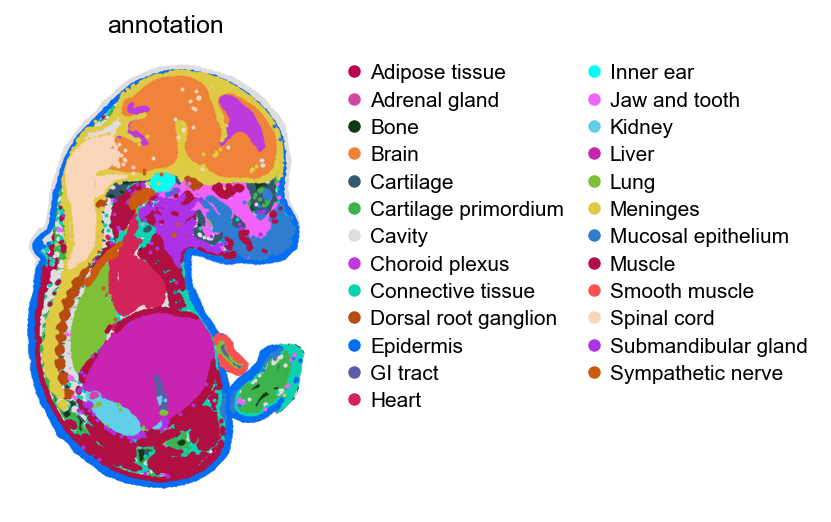
basis="spatial" is the only thing that differs from a UMAP call — the
embedding here is physical position, so the plot is the tissue.
2. Markers per organ
The grouping is annotation; everything else is
chapter 1.
res = cosg.run_cosg_cytome( ds, groupby="annotation", layer="data", # this file stores normalised values mu=100, n_genes_user=30, calculate_pvalues=True, output_format="ndarray",)markers = pd.DataFrame(res["names"], columns=list(res["groups_order"]))markers[["Brain", "Liver", "Muscle", "Cartilage"]].head(3) Brain Liver Muscle Cartilage0 Lhx9 Ermap Gm28653 Sp71 Tbr1 Gm20425 Neb Panx32 Gad2 Hemgn Trim55 Ifitm5Forty seconds for 121,767 bins, streamed off disk.
These are the right genes, which is the point of running it on annotated data first: Tbr1 and Gad2 are canonical cortical excitatory and inhibitory markers; Hemgn (hemogen) is erythroid, and at E16.5 the liver is the haematopoietic organ; Neb (nebulin) is a sarcomeric protein; Sp7 (osterix) is the master osteoblast transcription factor.
3. Plot them back onto the tissue
This is the check that dissociated data cannot give you.
genes = [markers[g][0] for g in ("Brain", "Liver", "Muscle", "Cartilage")]piaso.pl.plotEmbedding(ds, color=genes, basis="spatial", point_size=0.6, layer="data", ncols=4)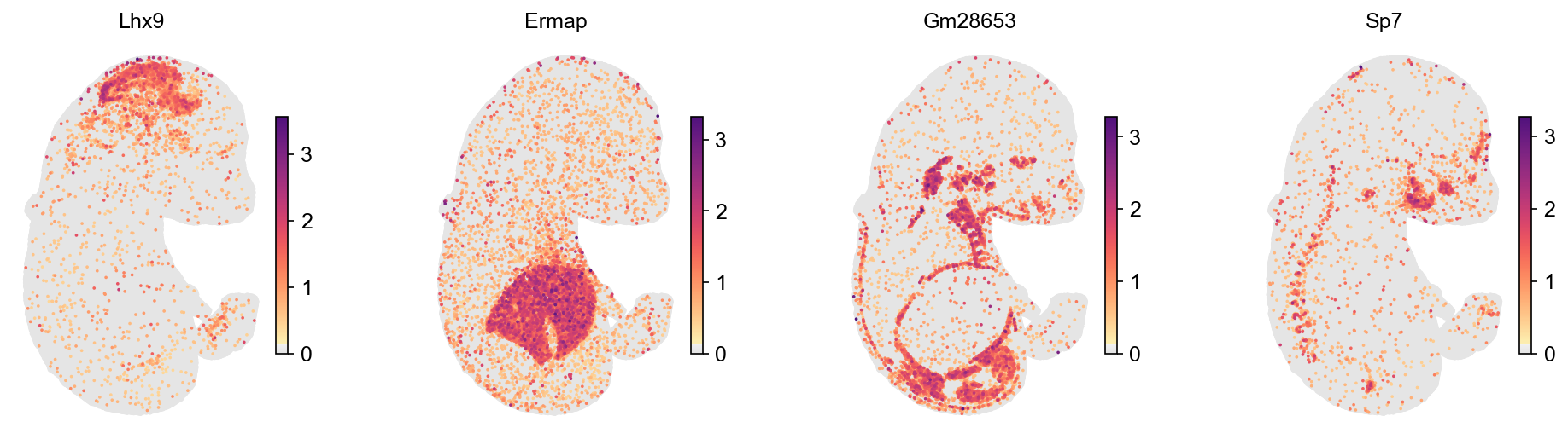
Each gene lands where it should. Lhx9 fills the brain and nothing else. Ermap, an erythroid membrane protein, fills the fetal liver. Gm28653 traces the intercostal and body-wall musculature. Sp7 draws the skeleton — the vertebral column, ribs and developing facial bones — as a thin line of ossifying cells, which is a shape no clustering told COSG about.
That last panel is worth pausing on: cartilage is 5,602 of 121,767 bins, arranged as a one-bin-wide sheet rather than a blob, and its top marker still comes out as the correct osteoblast gene.
4. Significance on spatial data
calculate_pvalues=True behaves exactly as in
chapter 1, and
the double-dipping caveat applies with one spatial twist worth stating.
The annotations used here are from the atlas, derived independently of this section’s expression matrix, so the p-values are valid as reported. If instead you cluster the bins on expression and then test markers of those clusters, you are double dipping in the ordinary way — and the fact that the clusters look anatomically convincing is not evidence against it, because spatially autocorrelated noise also looks convincing.
Spatial data adds a second caveat that the p-values do not address: neighbouring bins are not independent observations. The exchangeability null treats bins as exchangeable, which is right for “is this gene associated with this annotation” and wrong if you intend the p-value to describe a spatial process. For spatial dependence as the object of study, see LARIS, which models it directly.
5. Other spatial platforms
Nothing above is Stereo-seq specific. The grouping is a column and the plot is an embedding, so the same three calls work on Xenium, MERFISH or Visium:
- Xenium + image overlay
- MERFISH sections
- Stereo-seq embryo — where this cytome is built
For a Visium object the bins are spots and annotation is usually a
deconvolution result, in which case remember that the labels came from a model
fitted to this same matrix — the double-dipping section applies.
Where to go next
- Regulons on a spatial section — from marker genes to the factors driving them.
- LARIS — spatial ligand–receptor analysis on the same kind of object.
- COSG on the GPU — for sections larger than this one.