Spatial: MERFISH sections in one cytome

MERFISH measures single molecules in intact tissue — no tissue photograph is part of the standard output, so this tutorial shows the imageless spatial path: many sections in one .cytome, section-wise panels, and coordinate queries. Data: the Moffitt et al. (2018) mouse hypothalamic preoptic atlas (73,655 cells × 161 genes), as packaged by squidpy.

1. Data

curl -L -o merfish.h5ad https://ndownloader.figshare.com/files/28169379

2. Sections into one file

import anndata as ad
import pandas as pd
import cytome
import piaso

a = ad.read_h5ad("merfish.h5ad")           # obs: Animal_ID, Bregma, Cell_class...

bregmas = sorted(a.obs.loc[a.obs["Animal_ID"] == 1, "Bregma"].unique())[:3]
sel = a[(a.obs["Animal_ID"] == 1) & a.obs["Bregma"].isin(bregmas)].copy()
sel.obs["section"] = pd.Categorical([f"bregma_{b:.2f}" for b in sel.obs["Bregma"]])

ds = cytome.from_anndata(sel, output="merfish_demo.cytome")   # 19,428 cells, 9 MB
piaso.settings.set_figure_params(style="cell")   # one house style across every figure

obsm['spatial'] becomes the spatial embedding and the R*-tree coordinate index automatically.

3. One panel per section

piaso.pl.plot_embeddings_split(ds, color="Cell_class", splitby="section",
                               basis="spatial", ncol=3)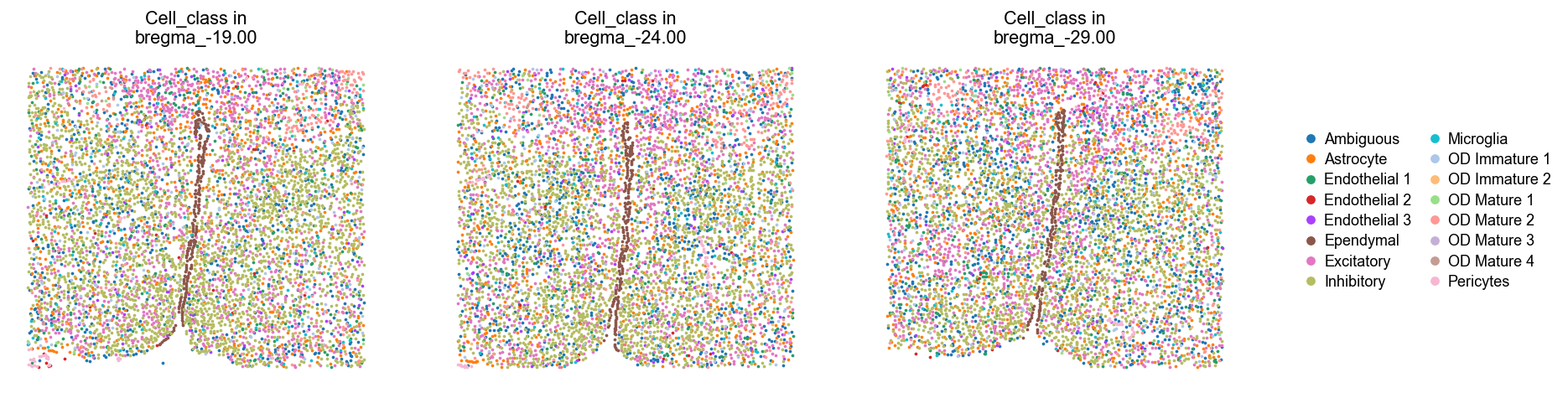

Without an image the axes keep the ordinary y-up orientation; the moment a panel has a stored image (image=True), it follows the image’s top-down convention instead — the two never mix.

4. Coordinate queries

The same indexed rectangle query works with or without images:

ds.cells_in_region(x=(-1000, 1000), y=(-1000, 1000))   # cell indices, sorted

For imaging platforms that do produce a picture (a DAPI or ssDNA registration), add it with ds.add_spatial_image(...) and every plot above accepts image=True — see the Xenium tutorial.

Marker genes in tissue coordinates

The panel is 161 genes, so every one is a marker someone chose. Plotting them on the coordinates is the fastest read of whether a section is what you think it is:

for g in ["Gad1", "Slc17a6", "Aqp4", "Mbp"]:
    piaso.pl.plotEmbedding(ds, color=g, basis="spatial",
                           vmin_pct=5, vmax_pct=95)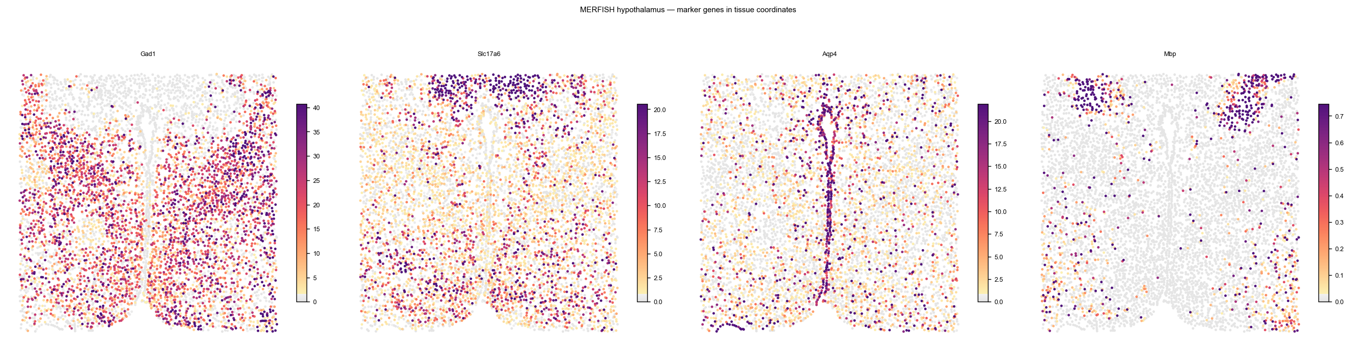

vmin_pct/vmax_pct clip the colour range to percentiles, which matters here: a handful of very bright cells otherwise own the scale and everything else washes out.

Four genes, four anatomies, none of them supplied: Gad1 across the inhibitory hypothalamus, Slc17a6 in the dorsal excitatory band, Aqp4 tracing the third ventricle as a single-cell-wide midline stripe, and Mbp in the fibre tracts at the top. The Aqp4 stripe is the check worth keeping — if the ependymal lining is not a clean line, the section or the registration is off.

One panel per cell class

The coordinates are already in a common frame here, so a split needs no alignment:

piaso.pl.plot_embeddings_split(ds, color="Cell_class", splitby="Cell_class",
                               basis="spatial", ncols=5)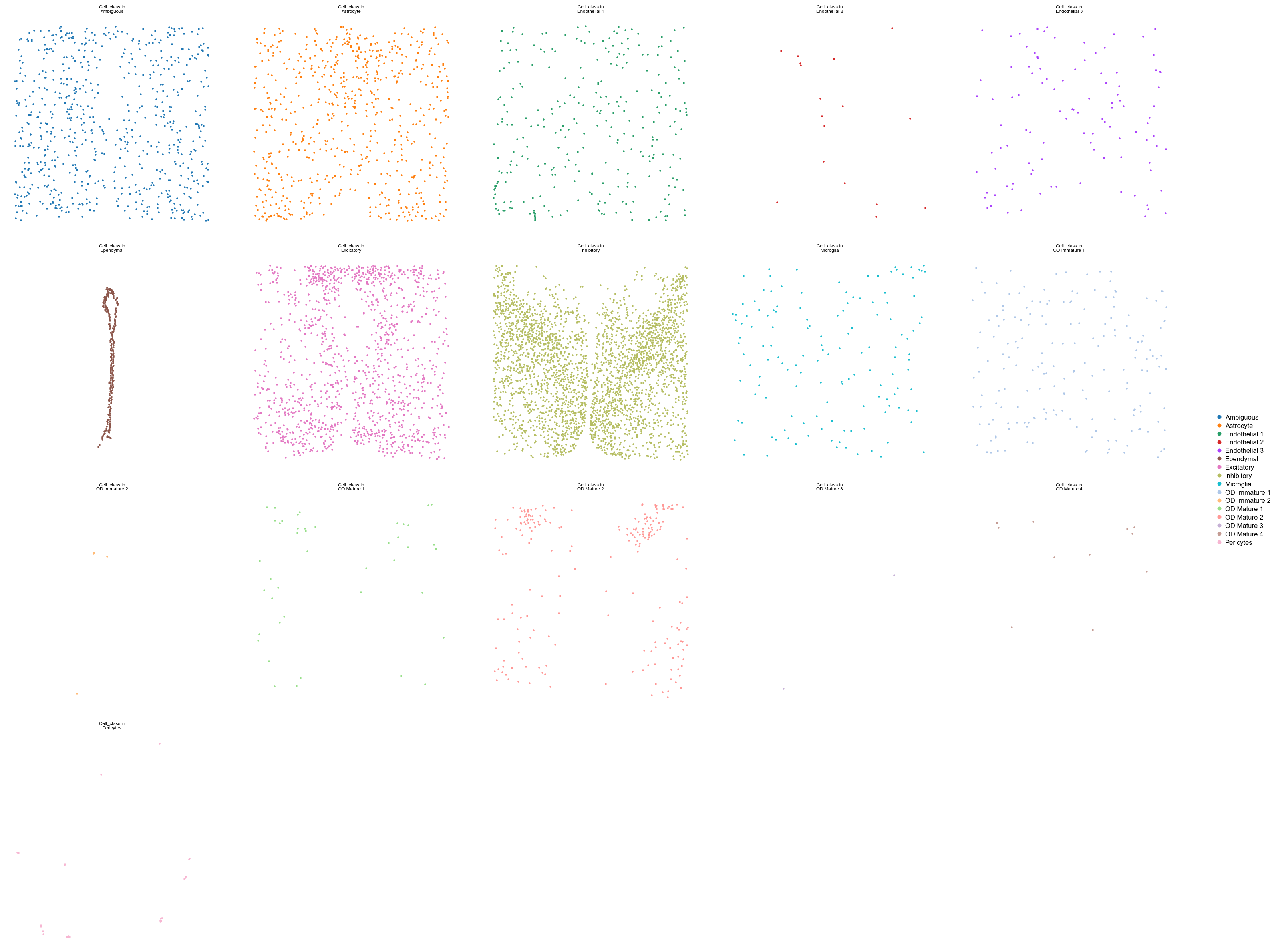

Sixteen classes, each on its own copy of the section. Inhibitory and excitatory neurons partition dorsoventrally, astrocytes and ependymal cells pick out the ventricle, and the mature oligodendrocyte classes sit in the tracts — the same story the gene panels tell, now per annotated class.

If your sections are not in a common frame — different chips, different stage positions — centre them first with piaso.pp.alignSpatialCoordinates(ds, batch_key="sample"), or each panel renders at its own offset.