Two preparations of one tissue: cells vs nuclei

The PBMC multi-sample tutorial found no batch effect between two libraries and therefore corrected nothing. This one is the other case: the same tissue — E18 mouse brain — prepared as whole cells and as nuclei. That is a real technical difference, it is large, and you can see exactly which biology it comes from.

import anndata
import pandas as pd
import piaso
import cosg

piaso.settings.set_figure_params(style="cell")

1. Load both preparations

parts = []
for name, label in (("e18_v3_cell", "cells"), ("e18_v3_nuclei", "nuclei")):
    a = piaso.data.load_dataset(name)
    a.obs["prep"] = label
    a.var_names_make_unique()
    parts.append(a)

adata = anndata.concat(parts, join="inner", index_unique="-")
del parts
adata.obs["prep"].value_counts()

11,843 whole cells and 5,973 nuclei, 29,836 genes in common.

2. Where the difference comes from

piaso.pp.calculateCellMetrics(adata, prefix_vars={"mt": "mt-",
                                                  "ribo": ["Rps", "Rpl"]})
adata.obs.groupby("prep", observed=True).agg(
    median_genes=("n_genes", "median"),
    median_counts=("n_counts", "median"),
    median_pct_mt=("pct_counts_mt", "median"),
    median_pct_ribo=("pct_counts_ribo", "median"),
)

prep	median genes	median counts	median % mito	median % ribo
cells	2,647	6,523	5.9	10.9
nuclei	1,796	3,620	11.3	1.9

The ribosomal fraction is the clean discriminator, and it is mechanistic: ribosomal protein transcripts are cytoplasmic, and a nuclei prep discards the cytoplasm. 10.9% against 1.9% is not a threshold artefact, it is the difference between the two protocols.

Two consequences worth stating:

A single QC threshold is wrong here. Nuclei have fewer genes by construction; min_features tuned on the cell library removes real nuclei.
Mitochondrial percentage does not behave as expected. Nuclei show the higher median (11.3% vs 5.9%), which is the opposite of the usual assumption. Ambient mitochondrial RNA is a plausible explanation, but the point for a tutorial is narrower: check the number rather than assume the direction.

piaso.pl.plot_features_violin(
    adata, ["n_genes", "n_counts", "pct_counts_mt", "pct_counts_ribo"],
    groupby="prep")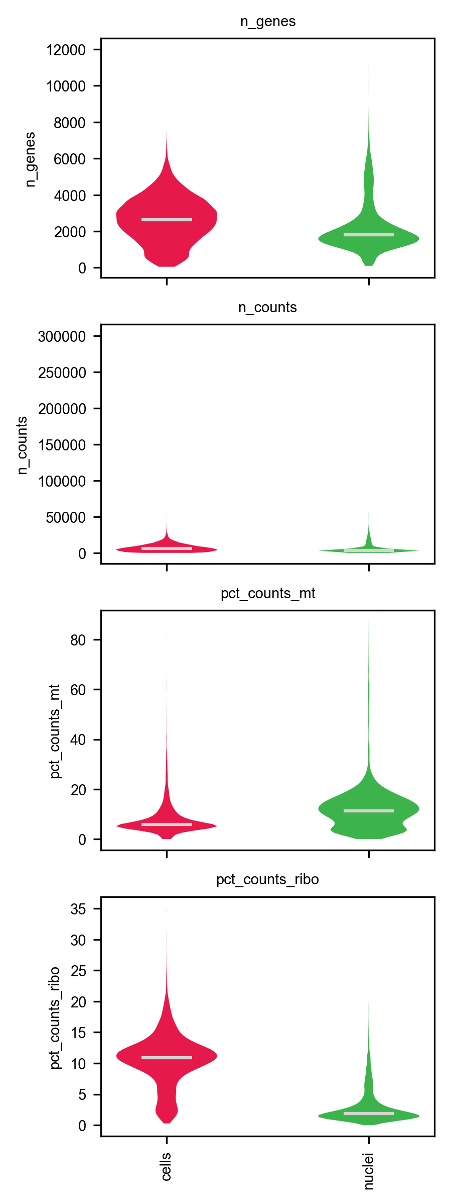

3. Doublets, per library

piaso.pp.scrublet(adata, library_key="prep", expected_doublet_rate=0.06,
                  random_state=0)
adata = adata[~(adata.obs["is_doublet"]
                | (adata.obs["scrublet_score"] > 0.3))].copy()
piaso.pp.filter_cells(adata, min_counts=500, min_features=250)
adata.shape

17,816 → 17,252 cells.

4. The batch effect, measured

piaso.tl.infog(adata, n_top_genes=3000)
piaso.tl.runSVD(adata, layer="infog", n_components=50, key_added="X_svd")
piaso.tl.neighbors(adata, use_rep="X_svd", n_neighbors=15)
piaso.tl.leiden(adata, resolution=1.0, key_added="leiden_svd")
piaso.tl.umap(adata, use_rep="X_svd")
adata.obsm["X_umap_svd"] = adata.obsm["X_umap"].copy()

piaso.pl.embedding(adata, basis="X_umap_svd", color="prep")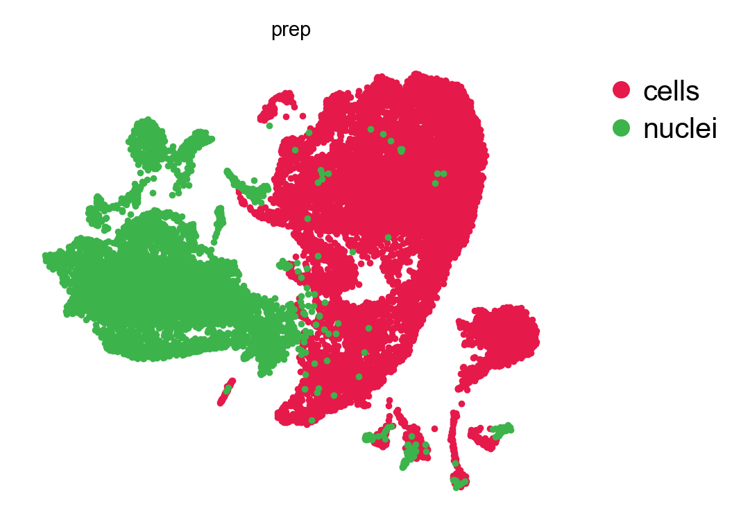

from sklearn.metrics import silhouette_score
silhouette_score(adata.obsm["X_svd"], adata.obs["prep"],
                 sample_size=4000, random_state=0)

0.322 — against −0.0003 for the two PBMC libraries. The preparations separate, and 30 Leiden clusters form on that separated space: the median cluster is 93% one preparation. Cluster structure here is partly protocol, not biology.

5. GDR

piaso.tl.runGDR(adata, batch_key="prep", groupby=None, layer="infog",
                infog_layer=None, score_layer="infog",
                n_gene=30, key_added="X_gdr")
piaso.tl.neighbors(adata, use_rep="X_gdr", n_neighbors=15)
piaso.tl.leiden(adata, resolution=1.0, key_added="leiden_gdr")
piaso.tl.umap(adata, use_rep="X_gdr")
adata.obsm["X_umap_gdr"] = adata.obsm["X_umap"].copy()

piaso.pl.embedding(adata, basis="X_umap_gdr", color="prep")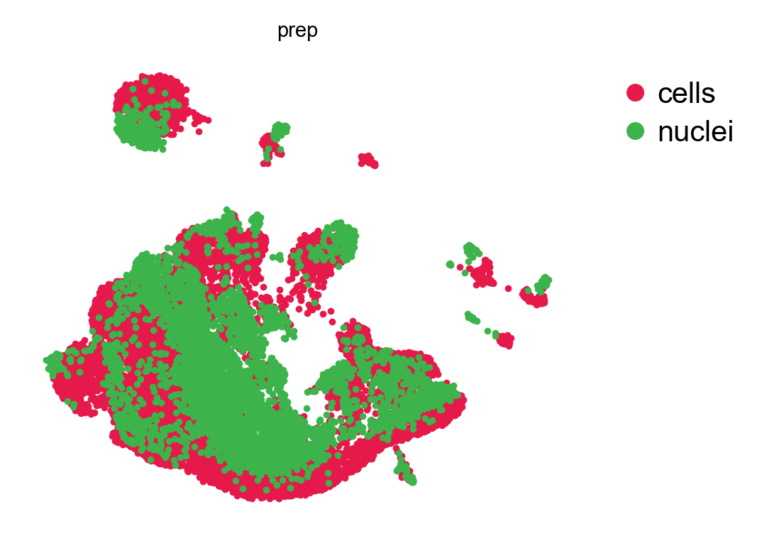

	clusters	silhouette, prep	median cluster’s majority-prep share
SVD	30	0.322	0.93
GDR	26	0.016	0.67

A twentyfold reduction, 0.322 → 0.016, without a batch-correction step: batch_key makes GDR select its marker genes within each library, so a gene that is specific only because of the preparation never becomes an axis. The ribosomal genes that separate the two protocols are exactly that kind of gene.

Note the residual: the median GDR cluster is still 67% one preparation, and some clusters remain nearly pure. That is not all failure — a whole-cell and a nuclei prep of the same tissue really do recover different proportions, and forcing them to 50/50 everywhere would be over-correction.

piaso.pl.embedding(adata, basis="X_umap_gdr", color="leiden_gdr",
                   legend_loc="both")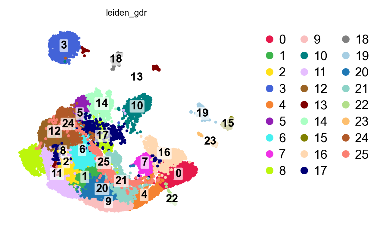

6. Annotation: match the reference to the stage

E18 cortex is mid-neurogenesis. Most of these cells are not yet any adult cell type, so the reference has to be a developmental one — see which studies exist:

piaso.tl.getMarkers(list_studies=True)

AllenDevVisualCortex2025_RNA is a developing mouse cortex atlas, which is the matched reference here. as_dict=True returns both the marker table and a {cell type: [genes]} dictionary, so unpack the two:

markers_df, marker_db = piaso.tl.getMarkers(
    study="AllenDevVisualCortex2025_RNA", as_dict=True)
len(marker_db), len(markers_df)

148 cell types, 7,400 marker rows. Keep the types that still have enough genes after intersecting with this object’s var_names — a type represented by two surviving genes is scored on almost no evidence:

covered = {ct: [g for g in genes if g in adata.var_names]
           for ct, genes in marker_db.items()}
covered = {ct: genes for ct, genes in covered.items() if len(genes) >= 5}
len(covered)

All 148 survive here. Now annotate, once per embedding, so the two can be compared on the same labels:

for tag, rep in (("svd", "X_svd"), ("gdr", "X_gdr")):
    piaso.tl.predictCellTypeByMarker(adata, marker_gene_set=covered,
                                     score_layer="infog", use_rep=rep,
                                     key_added=f"CellTypes_dev_{tag}")

adata.obs["CellTypes_dev_gdr"].value_counts().head(8)

cell type	cells
IMN IT Upper Layer	4,373
IMN IT Deep Layer	1,416
IMN nonIT	1,281
IP IT	1,039
MGE GABA	1,031
Glioblast SVZ	759
CGE GABA	605
Glioblast Astro	568

IMN is immature neuron, IP is intermediate progenitor, Glioblast is a glial precursor. That is what E18 cortex is made of, and it is a vocabulary an adult taxonomy does not contain at all — an adult reference has no label to give an intermediate progenitor, so it is forced to call it something else.

What changes against an adult reference

Running the same cells against AllenWholeMouseBrain_isocortex — an adult taxonomy — and crossing the two calls shows exactly where the adult one has to improvise:

adult call	developmental call	cells
L5 IT CTX Glut	IMN IT Upper Layer	997
L6 IT CTX Glut	IMN IT Upper Layer	740
Astro-TE NN	Glioblast SVZ	721
L5 IT CTX Glut	IMN nonIT	642
Sst Gaba	MGE GABA	544
Vip Gaba	CGE GABA	433

The interneurons survive the translation well — Sst maps to MGE, Vip to CGE, and those lineages are already specified at E18. The excitatory neurons do not: cells the adult reference splits into L5 IT, L6 IT, L5 ET and L4/5 IT are one population of upper-layer immature neurons that has not yet made that distinction. And “Astro-TE”, a mature astrocyte type, is a glioblast.

Neither call is a bug. The adult reference answers the only question it can — which adult type is this most like — and that is the wrong question at E18.

Plotting 121 labels

121 of the 148 types get at least one cell, which no single figure can show. Collapse the tail for display only; the annotation itself is unchanged:

import pandas as pd

frac = adata.obs["CellTypes_dev_gdr"].value_counts(normalize=True)
keep = list(frac[frac >= 0.01].index)          # 18 types, 80.6% of cells
for tag in ("svd", "gdr"):
    col = f"CellTypes_dev_{tag}"
    label = adata.obs[col].astype(str).where(adata.obs[col].isin(keep), "other")
    adata.obs[f"{col}_major"] = pd.Categorical(label, categories=keep + ["other"])

piaso.pl.embedding(adata, basis="X_umap_gdr", color="CellTypes_dev_gdr_major")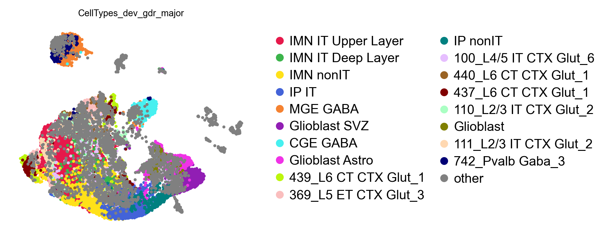

piaso.pl.plot_embeddings_split(adata, basis="X_umap_gdr",
                               color="CellTypes_dev_gdr_major", splitby="prep")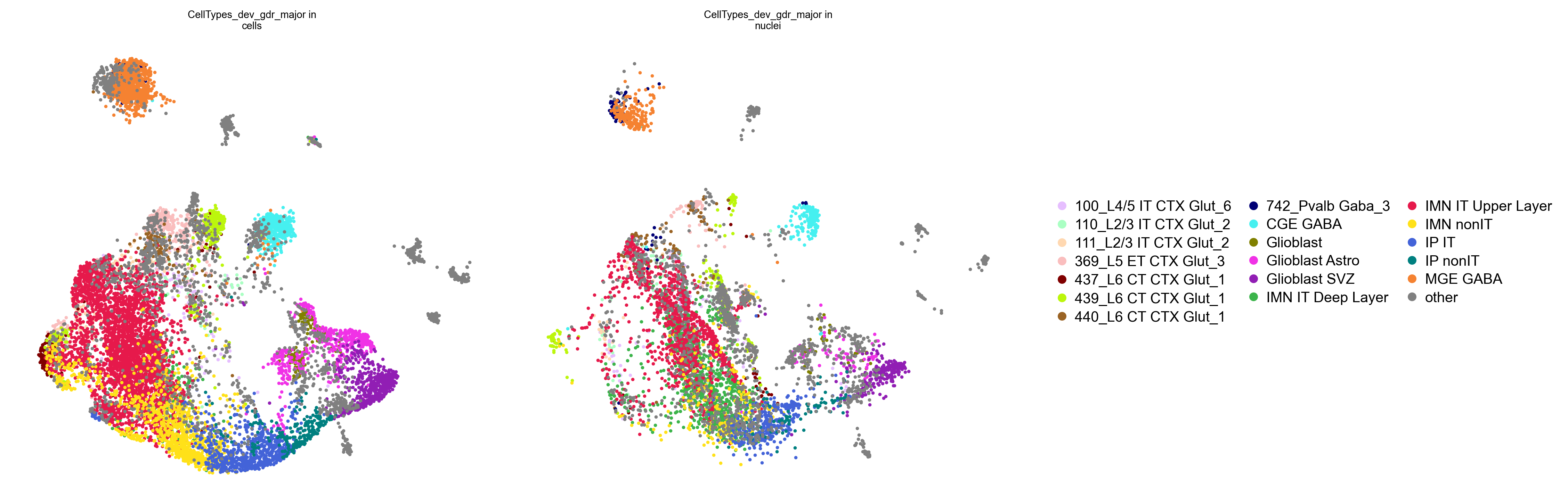

The honest caveat from the SVD/GDR comparison still holds. On these 19 display labels the cell-type silhouette is −0.169 for SVD and −0.023 for GDR — negative in both. Continuous differentiation does not produce compact separated clusters, and it should not be reported as if it did. GDR is the better of the two by a factor of seven, and that is the claim the numbers support.

top3, seen = [], set()
for ct in keep:
    picked = [g for g in covered[ct] if g not in seen][:3]
    top3 += picked; seen.update(picked)

sub = adata[adata.obs["CellTypes_dev_gdr_major"] != "other"].copy()
piaso.pl.dotplot(sub, top3, groupby="CellTypes_dev_gdr_major",
                 standard_scale="var")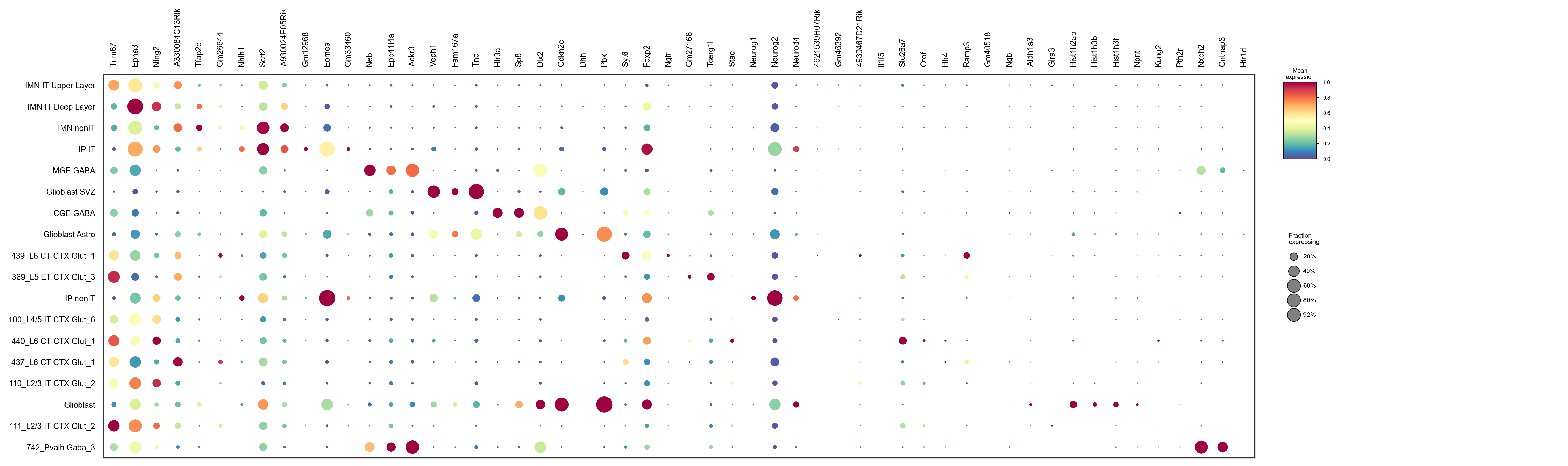

Worth checking one gene by hand before trusting the rest: Eomes (Tbr2) comes up for IP IT, and Eomes is the intermediate-progenitor marker in developing cortex. Neurog2 and Neurod4 land on the neurogenic populations, Dlx2 on the GABAergic ones, Sp8 on CGE. The reference is recovering mechanism, not just correlations.

When to reach for a batch correction

Between these two tutorials:

	PBMC SAN1/SAN2	E18 cells vs nuclei
prep/sample silhouette, SVD	−0.000	0.322
what to do	nothing	choose the embedding deliberately
GDR’s effect	better cell-type structure	20× less protocol separation

Measure before correcting. The number in step 4 is two lines and answers the question that the colours only hint at.