COSG across batches

A cosine score is computed over all the cells at once, which means the batch with the most cells has the most say. If one sample dominates a cell type — or if the samples were prepared differently — the top marker can be a gene that is specific to that sample’s version of the cell type, not to the cell type.

batch_key fixes this by scoring each batch separately and averaging the cosines. A gene now has to be specific in every batch to rank highly, instead of being specific in the largest one.

Marker genes — chapter 3 of 5

Chapter 1: markers and their significance — read this first · Chapter 2: COSG on a cytome · Chapter 4: COSG on the GPU · Chapter 5: COSG on spatial data

1. A dataset with real batch structure

The adult cortex Multiome object was generated with five nuclei-isolation protocols, recorded in adata.obs['Sample']:

import numpy as np
import pandas as pd
import piaso, cosg

adata = piaso.data.load_dataset("adult_cortex_multiome_rna")
adata.X = adata.layers["log1p"].copy()
adata.obs["Sample"].value_counts()

1c_TST_NP40_004                5071
1c_UC                          4920
1c_TST                         4364
1c_without_permiabilization    2139
1c                              918

This is the awkward case rather than the easy one: the batches differ in protocol, not just in run date, so they differ both in which cells they captured and in how much ambient RNA came along.

import matplotlib.pyplot as plt

ct = pd.crosstab(adata.obs["CellTypes"], adata.obs["Sample"], normalize="columns")

fig, ax = plt.subplots(figsize=(7.2, 4))
bottom = np.zeros(ct.shape[1])
colors = plt.cm.tab20(np.linspace(0, 1, ct.shape[0]))
for i, cell_type in enumerate(ct.index):
    ax.bar(ct.columns, 100 * ct.loc[cell_type].values, bottom=bottom,
           color=colors[i], label=cell_type)
    bottom += 100 * ct.loc[cell_type].values

ax.set_ylabel("% of the batch")
ax.set_xticks(range(len(ct.columns)))
ax.set_xticklabels(ct.columns, rotation=45, ha="right", fontsize=7)
ax.legend(fontsize=5, ncol=2, bbox_to_anchor=(1.01, 1), loc="upper left",
          frameon=False)
fig.tight_layout()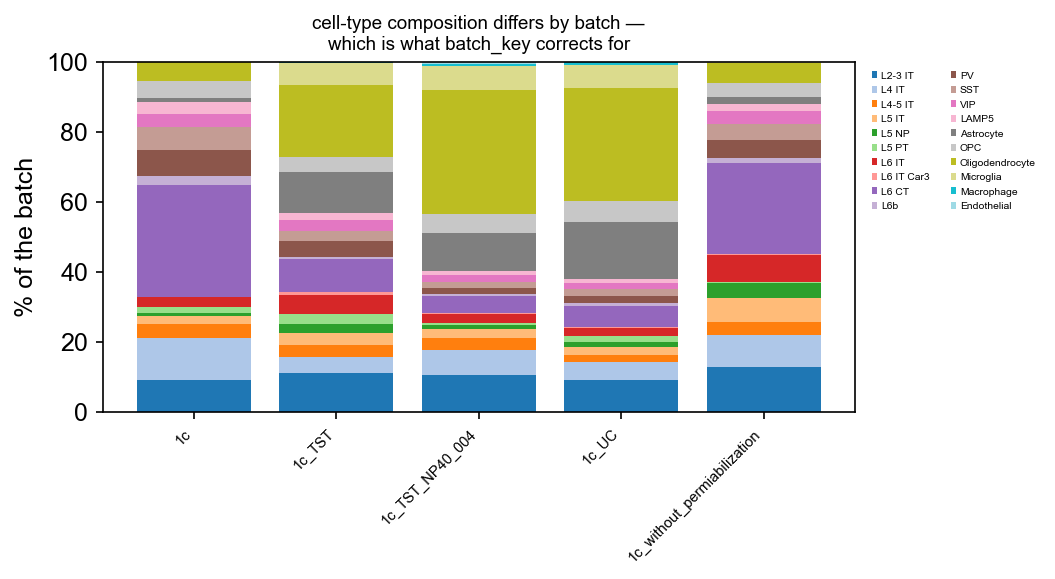

The protocol names are long enough to collide under the bars, so they are set at 45° with ha="right" — which anchors each label’s end under its own bar rather than centring it across two.

The composition is visibly uneven — the unpermeabilised sample has a very different mix from the TST ones. That imbalance is the mechanism: a cell type that is 60% one sample gets its markers chosen largely by that sample.

2. Turning it on

cosg.cosg(adata, groupby="CellTypes", key_added="cosg_batch",
          mu=100, n_genes_user=50,
          batch_key="Sample",
          batch_cell_number_threshold=5)

One second on this object — the stratification costs essentially nothing, because it is the same arithmetic run once per batch on smaller matrices.

batch_cell_number_threshold (default 3) is the important companion argument. If a cell type has fewer than this many cells in a batch, that batch’s cosine for that cell type is dropped from the average rather than contributing a number estimated from two cells. With 20 cell types and 5 batches, some combinations are genuinely empty — Endothelial has 41 cells in total — and without the threshold those near-empty cells would dominate the mean, since a cosine computed from a single cell is 1.0 by construction. Raise it when your batches are small and you want to be conservative — on this dataset the default is far too permissive, which §4 takes apart.

3. What actually changes

Comparing the two marker tables, cell type by cell type:

plain   = pd.DataFrame(adata.uns["cosg"]["names"])
batched = pd.DataFrame(adata.uns["cosg_batch"]["names"])

overlap = {c: len(set(plain[c][:20]) & set(batched[c][:20])) / 20
           for c in plain.columns}
np.mean(list(overlap.values()))

0.86

order = sorted(overlap.items(), key=lambda kv: kv[1])

fig, ax = plt.subplots(figsize=(6.4, 3.8))
ax.bar([k for k, _ in order], [100 * v for _, v in order],
       color="#009E73", width=.65)
ax.set_ylabel("top-20 markers kept (%)")
ax.set_xticks(range(len(order)))
ax.set_xticklabels([k for k, _ in order], rotation=45, ha="right", fontsize=7)
fig.tight_layout()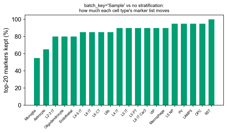

86% of the top-20 markers are unchanged, which is the reassuring answer: the batch effect here is real but not catastrophic, and most markers are specific in every batch. The interesting part is the tail:

cell type	top-20 kept
Microglia	55%
Astrocyte	65%
L2-3 IT	80%
Oligodendrocyte	80%
Endothelial	80%

Microglia and astrocytes move most, and that is not a coincidence — they are the types most sensitive to dissociation, which is exactly what these five protocols differ in. The genes that drop out of their lists are the ones whose apparent specificity came from one protocol.

Looking at one cell type’s scores

The overlap counts genes going in and out of a list, which does not say whether the scores changed a little or a lot. Microglia moved most, so take it apart.

Both runs are scored over every gene and then IQR-normalised before comparing. That step is not optional here: batch_key averages per-batch cosines, which changes the scale of the score itself, so the raw numbers from the two runs are not on the same axis.

for key, extra in (("plain", {}),
                   ("batched", dict(batch_key="Sample",
                                    batch_cell_number_threshold=5))):
    cosg.cosg(adata, groupby="CellTypes", key_added=f"cosg_all_{key}",
              mu=100, n_genes_user=adata.n_vars, **extra)

n_plain = cosg.iqrLogNormalize(cosg.indexByGene(
    pd.DataFrame(adata.uns["cosg_all_plain"]["COSG"])))
n_batch = cosg.iqrLogNormalize(cosg.indexByGene(
    pd.DataFrame(adata.uns["cosg_all_batched"]["COSG"])))

a, b = n_plain["Microglia"], n_batch["Microglia"]
a.corr(b), a.corr(b, method="spearman")

(0.9961, 0.9932)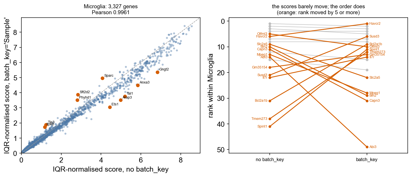

The scores are almost unchanged — Pearson 0.996 over 3,327 genes — while 45% of the top 20 turned over. Both statements are true, and together they say what batch_key actually does here.

The reason is in the numbers: the top 20 Microglia genes score between 7.67 and 8.55. They are near-ties. A shift far too small to see on the left panel is more than enough to reorder them, which is why the right panel — the same genes by rank — looks so much more dramatic than the scatter beside it.

Do not read a small rank change as a finding. Between two genes separated by 0.05 normalised units the order is arbitrary, and either run could produce either. If you need a stable list, take the union of both runs rather than believing the top of one.

That is how to read the previous plot on your own data: the ranking is a diagnostic.

4. Why those genes moved, and why the threshold matters more than it looks

The five biggest demotions — Gngt2, Arap3, Tal1, Ets1, Anxa3 — have something in common, and it is not biology. Count the Microglia in each batch:

adata.obs.loc[adata.obs["CellTypes"] == "Microglia", "Sample"].value_counts()

1c_TST_NP40_004                352
1c_UC                          319
1c_TST                         279
1c_without_permiabilization      8
1c                               0

One batch holds 8 Microglia. All five demoted genes are detected in 0% of those 8 cells, and batch_key averages the per-batch cosines with equal weight — so a batch of 8 counts exactly as much as a batch of 352, and a gene those 8 cells happen to miss loses a quarter of its score.

batch_cell_number_threshold=5 let that batch in, because 8 ≥ 5. Raising it to 50 drops it, and the demoted genes come back:

for thr in (5, 50):
    cosg.cosg(adata, groupby="CellTypes", key_added=f"thr{thr}", mu=100,
              n_genes_user=adata.n_vars, batch_key="Sample",
              batch_cell_number_threshold=thr)

gene	no batch_key	thr=5	thr=50	rank: none → 5 → 50
Anxa3	5.84	4.49	7.68	159 → 238 → 49
Tal1	5.20	3.77	7.33	222 → 308 → 100
Arap3	4.99	3.52	6.91	239 → 344 → 159
Gngt2	6.83	5.36	6.93	72 → 169 → 157
Selplg	8.55	8.41	8.15	1 → 2 → 3
Tmem119	8.40	8.13	7.97	3 → 5 → 17
Csf3r	8.14	7.92	7.95	7 → 7 → 19

Read the last two rows before concluding that thr=50 is the right answer. Excluding the small batch does not simply undo a distortion — it also pushes the canonical markers down (Tmem119 3 → 17, Csf3r 7 → 19), and the top-20 overlap with the unstratified run falls from 0.55 to 0.30. Neither setting is the true one; they weight the evidence differently, and the marker list is genuinely sensitive to that choice.

The practical rule: set batch_cell_number_threshold from the size of the group you are willing to let vote, not from the default. The default of 3 is permissive enough that a handful of cells can outvote several hundred. A reasonable starting point is a threshold at which every included batch could plausibly estimate a cosine on its own — a few dozen cells — and then check, as above, that your canonical markers survive it.

This is also the honest reason the marker lists in §3 moved by 14% overall rather than not at all. Some of that is the batch effect being corrected. Some of it is an 8-cell batch being given a full vote. A cell type near 100% has markers that do not care about your batches. A cell type well below it is telling you that its unstratified marker list was partly describing a batch, and the stratified one is the safer table to publish.

5. Significance under stratification

calculate_pvalues=True works with batch_key, and the null changes to match: labels are permuted within batch, so the statistic becomes a sum of independent per-stratum sums. The moments and the saddlepoint tail are computed per stratum and combined.

cosg.cosg(adata, groupby="CellTypes", key_added="cosg_batch",
          mu=100, batch_key="Sample", calculate_pvalues=True)

This is the right null when your grouping is confounded with batch, and it is stricter — a gene that looks significant only because one batch is enriched for one cell type no longer is.

Two limits worth knowing:

• pvalue_method='exact' declines under stratification. The exact polynomial tail enumerates one hypergeometric null; a stratified null is a convolution of several, which it does not enumerate. It falls back to the saddlepoint and says so.
• On the streaming path, batch_key together with calculate_pvalues=True raises. Run the markers streamed and, if you need stratified p-values, the significance step in memory on the subset you care about.

The double-dipping caveat from chapter 1 is untouched by any of this. Stratifying by batch corrects for batch; it does not make labels derived from this matrix legitimate.

6. When not to use it

batch_key is not free of assumptions. It assumes every batch is measuring the same underlying cell type, so averaging their cosines is meaningful. Two cases where that is wrong:

• The “batch” is a condition. If your batches are control and treated, a gene that responds to treatment is not a batch artefact, and averaging over the two hides it. Stratify by the technical variable, not the biological one.
• A cell type exists in only one batch. Its average is then computed from that single batch anyway, and batch_cell_number_threshold will have dropped the others — the result is correct but carries no cross-batch evidence, so treat it as you would an unstratified run.

If your batch effect is severe enough that the cell types do not overlap across batches, the fix is upstream: integrate first — see GDR — and run COSG on the harmonised labels.

Where to go next

• Markers and their significance — the columns, and what mu does.
• COSG on a cytome — the same run without loading the matrix.
• COSG on the GPU — the speed axis, measured.