Multiple samples: QC, embedding and annotation

Everything in the single-sample tutorial still applies. Three things change once there is more than one library, and each has a step of its own here:

1. doublets are per library — a barcode is only a doublet relative to the pool it was loaded with;
2. QC thresholds are per library — libraries differ in depth, and one global cut silently removes more of the shallower one;
3. the embedding is worth choosing deliberately — and whether it needs a batch correction at all is a question to measure, not to assume.

We use two human PBMC snMultiome libraries, SAN1 and SAN2 (De Rop et al. 2024). Only the RNA side is used here.

import anndata
import pandas as pd
import piaso
import cosg

piaso.settings.set_figure_params(style="cell")

Two routes. This page concatenates AnnData objects in memory, which is right for a handful of libraries. The other merges them into one cytome and never holds the matrix whole — Multiple samples, in a cytome. Same method; the difference only starts to matter at tens of samples.

1. Load and concatenate

parts = []
for name in ("pbmc_multiome_san1", "pbmc_multiome_san2"):
    a = piaso.data.load_dataset(name)
    a.obs["sample"] = name.rsplit("_", 1)[-1].upper()
    a.var_names_make_unique()
    parts.append(a)

adata = anndata.concat(parts, join="inner", index_unique="-")
del parts
adata.obs["sample"].value_counts()

3,545 cells from SAN1 and 4,360 from SAN2, 36,601 genes in common. index_unique keeps barcodes distinct: the same barcode sequence occurs in both libraries and means different cells.

2. Quality control, per sample

groupby="sample" is the whole difference: the same metrics, split by library, so a library-specific problem is visible instead of averaged away.

piaso.pp.calculateCellMetrics(adata, prefix_vars={"mt": "MT-",
                                                  "ribo": ["RPS", "RPL"]})
piaso.pl.plot_features_violin(
    adata, ["n_genes", "n_counts", "pct_counts_mt", "pct_counts_ribo"],
    groupby="sample", ncol=2, width_single=3.4, height_single=3.0)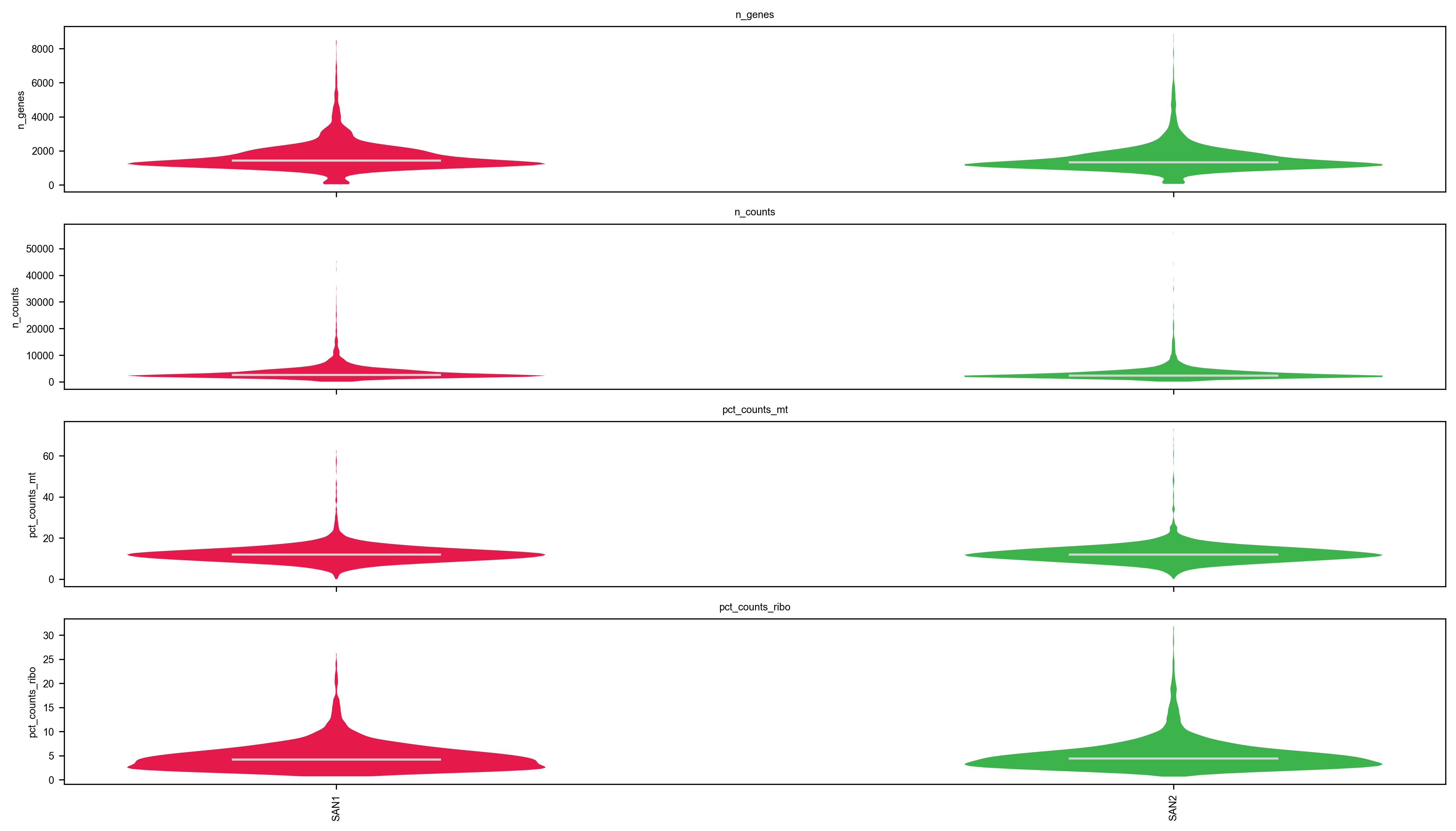

ncol=2 matters: four metrics in a single row makes a strip so wide the distributions are unreadable at page width. width_single/height_single size each panel rather than the whole grid.

Set thresholds after looking at this. If one library is systematically shallower, a single min_counts takes a bigger bite out of it, and the difference that survives into the clustering is technical.

3. Doublets, per library

Pass library_key. Scrublet simulates doublets by adding pairs of observed profiles together; cells from a library the barcode was never mixed with are not valid partners, so the simulation has to run within each library.

piaso.pp.scrublet(adata, library_key="sample", expected_doublet_rate=0.06,
                  random_state=0)

adata.obs.groupby("sample", observed=True).agg(
    called=("is_doublet", "sum"),
    n=("is_doublet", "size"),
    median_score=("scrublet_score", "median"),
)

adata = adata[~(adata.obs["is_doublet"]
                | (adata.obs["scrublet_score"] > 0.3))].copy()
piaso.pp.filter_cells(adata, min_counts=500, min_features=250)
adata.shape

7,905 → 6,740 cells.

4. Is there a batch effect at all?

The reflex is to reach for a batch correction. Measure first: correcting an effect that is not there costs real biological signal.

Save the raw counts before you normalise. piaso.tl.infog writes its result to adata.layers["infog"] and leaves adata.X alone, so nothing here destroys the UMIs — but nothing guarantees they survive either. One sc.pp.normalize_total later, in this notebook or the next one, overwrites X in place and they are gone for good. The line costs a copy and buys back every count-based analysis: differential expression, pseudobulk, re-normalising with different parameters, and writing an .h5ad a collaborator can still use.

adata.layers["counts"] = adata.X.copy()          # the raw UMIs, kept
piaso.tl.infog(adata, n_top_genes=3000)
piaso.tl.runSVD(adata, layer="infog", n_components=50, key_added="X_svd")
piaso.tl.neighbors(adata, use_rep="X_svd", n_neighbors=15)
piaso.tl.leiden(adata, resolution=1.0, key_added="leiden_svd")
piaso.tl.umap(adata, use_rep="X_svd")
adata.obsm["X_umap_svd"] = adata.obsm["X_umap"].copy()

piaso.pl.embedding(adata, basis="X_umap_svd", color="sample")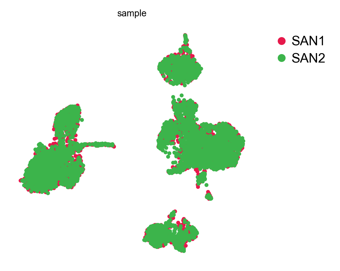

Colours interleave. Put a number on it with a silhouette score of the sample label in the embedding: near zero means the libraries are indistinguishable, positive means they separate.

from sklearn.metrics import silhouette_score
silhouette_score(adata.obsm["X_svd"], adata.obs["sample"],
                 sample_size=4000, random_state=0)

−0.0003. There is no batch effect between SAN1 and SAN2 to correct. That is not a general result — it is two libraries of the same tissue prepared the same way — but it is the answer for this data, and it means Harmony is not needed here. Reach for a correction when this number says you have something to correct.

5. GDR: a better embedding, not a correction

runGDR is a different way to build the embedding, not a batch fix. It selects marker genes per group and embeds cells on their scores, so the axes are cell-identity axes rather than directions of maximum variance.

batch_key makes the marker selection run per library, so a gene that only looks specific because of one library’s depth cannot drive the embedding. groupby=None lets GDR find its own groups; handing it a clustering that already contains the batch structure would defeat the point.

piaso.tl.runGDR(adata, batch_key="sample", groupby=None,
                layer="infog",          # normalized matrix to embed
                infog_layer=None,       # .X is already raw counts here
                score_layer="infog",    # score the marker sets on the same layer
                n_gene=30, key_added="X_gdr")
piaso.tl.neighbors(adata, use_rep="X_gdr", n_neighbors=15)
piaso.tl.leiden(adata, resolution=1.0, key_added="leiden_gdr")
piaso.tl.umap(adata, use_rep="X_gdr")
adata.obsm["X_umap_gdr"] = adata.obsm["X_umap"].copy()

piaso.pl.embedding(adata, basis="X_umap_gdr", color="sample")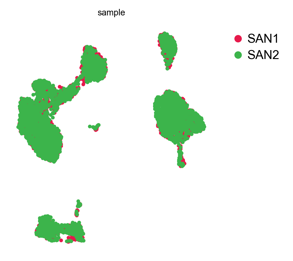

piaso.pl.embedding(adata, basis="X_umap_gdr", color="leiden_gdr",
                   legend_loc="both")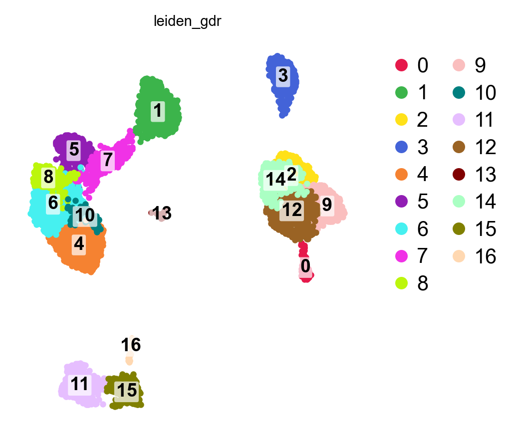

The comparison

Two silhouette scores, on the same cells, in each embedding: one for the sample label (lower is better — libraries mixed), one for the cell type label (higher is better — identities separated).

	clusters	silhouette, sample	silhouette, cell type	SAN1 fraction per cluster
SVD	17	−0.000	0.061	0.39 – 0.55
GDR	17	+0.001	0.170	0.36 – 0.54

Neither embedding separates the libraries: both sample silhouettes are zero to three decimal places. But GDR’s cell type silhouette is 2.8× higher: the same cells, the same clusters, arranged so that identity is what the geometry encodes. Cells from the two libraries sit together because they are the same cell type, which is what you want mixing to mean: not because a correction pushed them together.

That is the argument for GDR here. It is not doing batch correction; there is nothing to correct. It is building an embedding on cell identity, and identity is shared across libraries.

6. Annotation

Same call as the single-sample tutorial, with use_rep="X_gdr" so the smoothing runs in the embedding you are using. For human PBMC the matched PIASOmarkerDB study is the Allen Human Immune Health Atlas:

# as_dict=True returns the {cell type: [genes]} dictionary,
# which is what predictCellTypeByMarker takes.
marker_db = piaso.tl.getMarkers(
    study="AllenHumanImmuneHealthAtlas_L2", as_dict=True)
piaso.tl.predictCellTypeByMarker(adata, marker_gene_set=marker_db,
                                 score_layer="infog", use_rep="X_gdr",
                                 key_added="CellTypes_gdr")
adata.obs["CellTypes_gdr"].value_counts().head(8)

29 types, and the composition is a PBMC composition: CD14 monocyte 1,703, naive CD4 T 985, CD56dim NK 733, memory CD4 T 628, naive B 461, MAIT 381, CD16 monocyte 353, naive CD8 T 296.

piaso.pl.embedding(adata, basis="X_umap_gdr", color="CellTypes_gdr")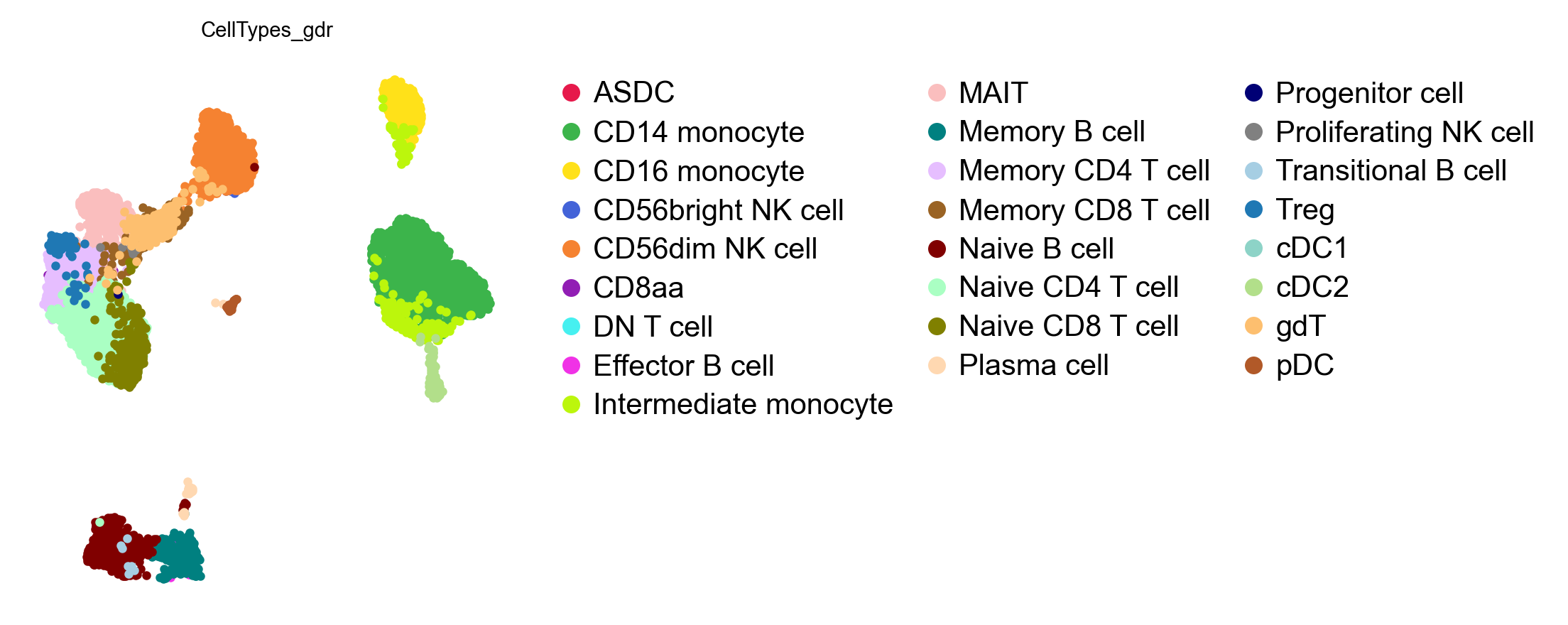

Split the same embedding by sample to see whether both donors contribute to every type:

piaso.pl.plot_embeddings_split(adata, basis="X_umap_gdr", color="CellTypes_gdr",
                               splitby="sample")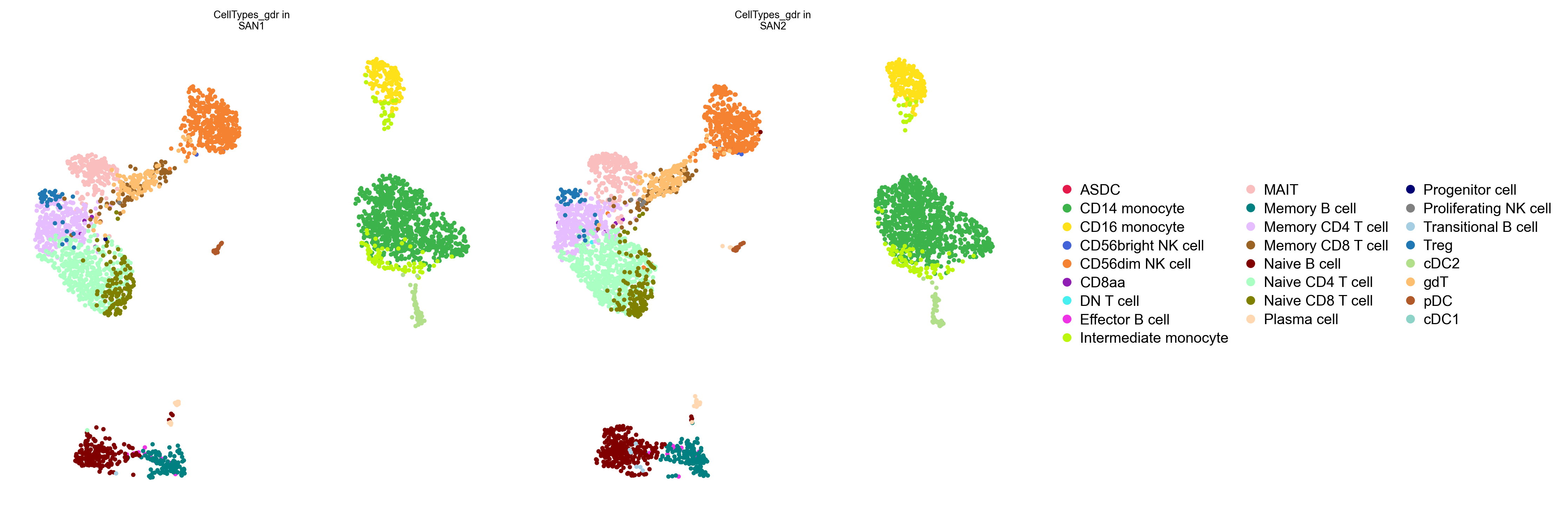

top3, seen = [], set()
for ct in adata.obs["CellTypes_gdr"].astype("category").cat.categories:
    picked = [g for g in marker_db[ct] if g in adata.var_names and g not in seen][:3]
    top3 += picked; seen.update(picked)

piaso.pl.dotplot(adata, top3, groupby="CellTypes_gdr", standard_scale="var")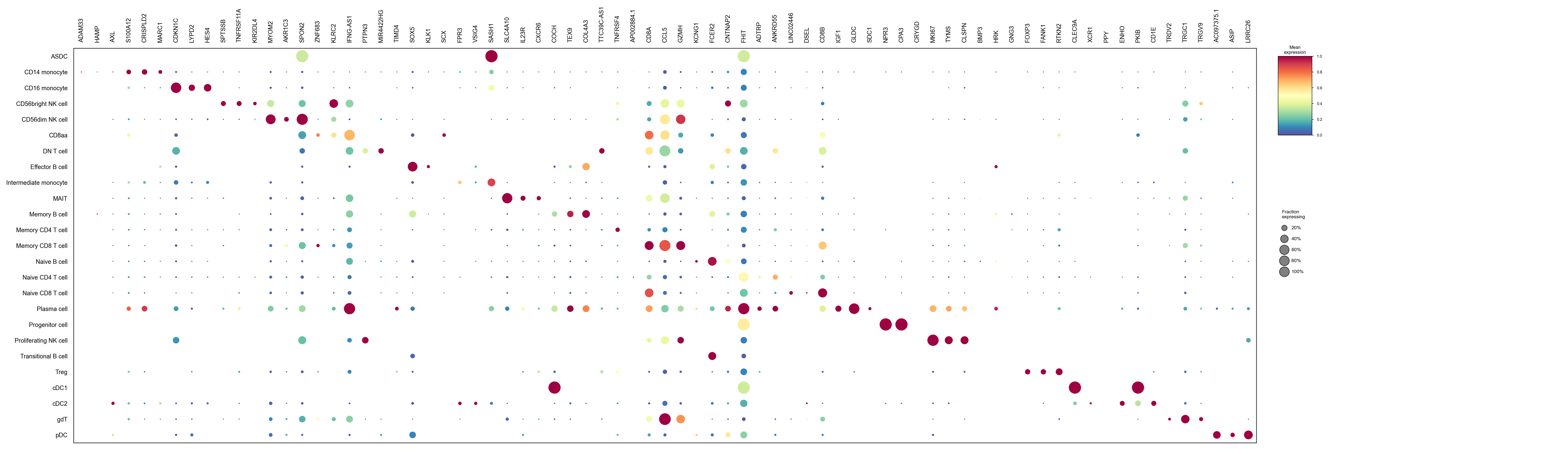

Where to go next

• More than two samples — nothing above changes. library_key and batch_key take any number of levels.
• A real batch effect — if the sample silhouette in step 4 is clearly positive, piaso.tl.runHarmony(adata, batch_key="sample", use_rep="X_svd") corrects the SVD in place; re-run neighbours, Leiden and UMAP on the result and check the number again.
• Streaming — the cytome tutorial applies here too; cytome.merge builds one file from several.
• Marker-gene-guided integration — piaso.tl.runGDR with batch_key, an alternative to correcting an SVD after the fact.