GDR on spatial transcriptomics: eight embryonic stages, 520,815 bins

Stage is a batch here in the awkward sense: E9.5 and E16.5 differ by real biology and by everything that changes when a section is nine days older. An embedding that separates the stages has told you nothing; one that mixes them while keeping organs apart is the useful one.

This runs INFOG → GDR → UMAP on the full MOSTA series — 520,815 bins × 23,761 genes, 45 organs, E9.5 to E16.5 — with batch_key="timepoint", entirely on disk.

1. INFOG from the raw layer

import piaso
import cytome, piaso

ds = cytome.open("allstage.cytome")
piaso.tl.infog(ds, modality="RNA", layer="count",
               key_added="infog", save_layer=True, inplace=True)
ds.flush(); ds.close()
piaso.settings.set_figure_params(style="cell")   # one house style across every figure

The layer is count, singular — MOSTA keeps raw counts there and normalized values in X, and after conversion the cytome carries RNA_count beside RNA_counts. INFOG refuses non-integer input rather than returning numbers that look fine, which is how you find out you passed the wrong one.

2. GDR with stage as the batch

piaso.tl.runGDR("allstage.cytome",
                batch_key="timepoint",      # the eight stages
                groupby="annotation",       # the 45 organs
                layer="infog", score_layer="infog",
                n_gene=20, mu=10.0, max_workers=16)

GDR finds marker genes per groupby category within each batch, scores every cell against them, and builds the embedding from those scores. Because the marker sets are derived per stage, a gene that marks brain at E10.5 and a gene that marks brain at E16.5 both contribute — the axis they define is “brain-ness”, not “stage”.

Nothing is loaded whole: the call takes the path, streams the matrix in chunks, and writes X_gdr back into the file.

ds = cytome.open("allstage.cytome")
ds.list_embeddings()      # ['RNA_spatial', 'X_gdr']

3. UMAP and what to look for

Order the stages once so every plot and groupby follows development rather than the alphabet (E10.5 sorts before E9.5 otherwise), then use PIASO’s own neighbours/UMAP rather than calling umap-learn by hand:

ORDER = ["E9.5","E10.5","E11.5","E12.5","E13.5","E14.5","E15.5","E16.5"]
ds.set_categories("timepoint", ORDER)        # stored in the cytome

piaso.tl.neighbors(ds, use_rep="X_gdr", n_neighbors=15)
piaso.tl.umap(ds, min_dist=0.3)              # writes X_umap into the file

piaso.pl.plotEmbedding(ds, color="timepoint",  basis="umap")
piaso.pl.plotEmbedding(ds, color="annotation", basis="umap")

timepoint is a numeric-looking label but a categorical column, so it gets a palette; a genuinely numeric column would get the diverging continuous map instead (Spectral_r), which is the default for cell-metadata values.

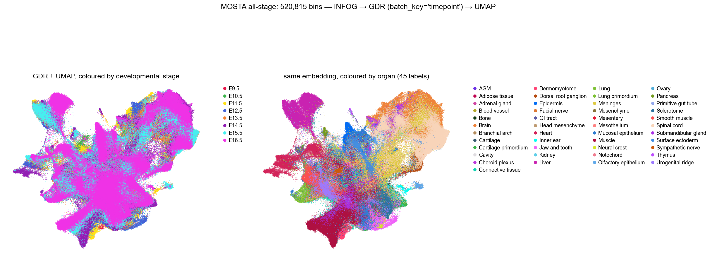
Read the two panels against each other — that comparison is the result:

By stage (left), the eight stages interleave across the whole embedding. There is no E9.5 island and no E16.5 island. E16.5 covers more of it simply because it contributes 121,767 of the 520,815 bins.
By organ (right), the same points resolve into contiguous territories: brain and spinal cord as one large block, liver, muscle, cartilage, meninges, epidermis each with their own.

Batch mixed, biology separated. Colouring by stage alone would look like a failure to integrate; colouring by organ alone would look like success without evidence. Both panels, same embedding, is the check.

3b. One panel per stage

The same embedding split by stage shows when each organ appears — the E9.5 panel is nearly all mesenchyme and neural tube, and organs fill in panel by panel:

piaso.pl.plot_embeddings_split(ds, color="annotation", splitby="timepoint",
                               basis="umap", ncols=4)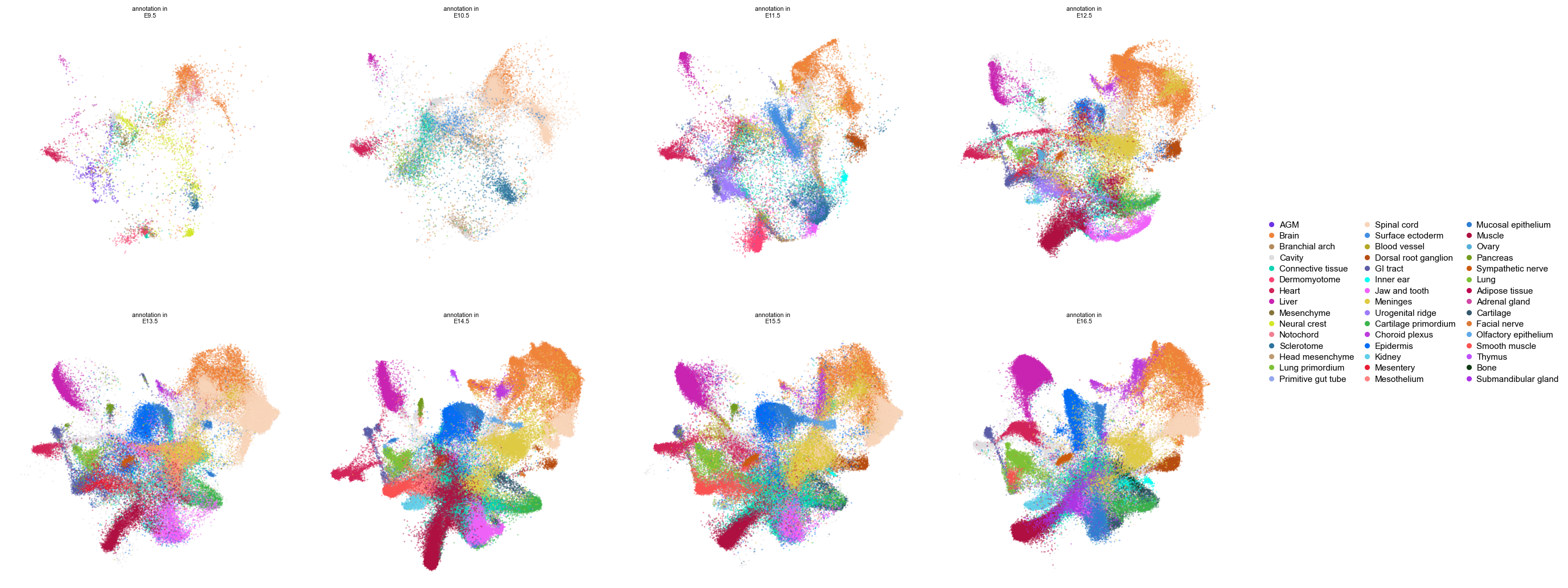

3c. Clusters back onto the tissue

Cluster the GDR embedding, then plot those clusters in spatial coordinates — the embedding never saw a coordinate, so anatomical structure in this plot is earned:

piaso.tl.neighbors(ds, use_rep="X_gdr", n_neighbors=15)   # if not already built
piaso.tl.leiden(ds, resolution=1.0, key_added="leiden_gdr")

piaso.pp.rotateSpatialCoordinates(ds, angle_degrees=90, spatial_key="spatial")
piaso.pp.alignSpatialCoordinates(ds, batch_key="timepoint",
                                 spatial_key="spatial",
                                 backup_spatial_key="spatial_raw")

# rotate to an upright section first -- alignment places sections, it does
# not orient them -- then centre each stage on its own centroid
piaso.pp.rotateSpatialCoordinates(ds, angle_degrees=90, spatial_key="spatial",
                                  backup_spatial_key="spatial_raw")
piaso.pp.alignSpatialCoordinates(ds, batch_key="timepoint",
                                 spatial_key="spatial",
                                 key_added="spatial_aligned")

piaso.pl.plot_embeddings_split(ds, color="leiden_gdr", splitby="timepoint",
                               basis="spatial_aligned", ncol=4)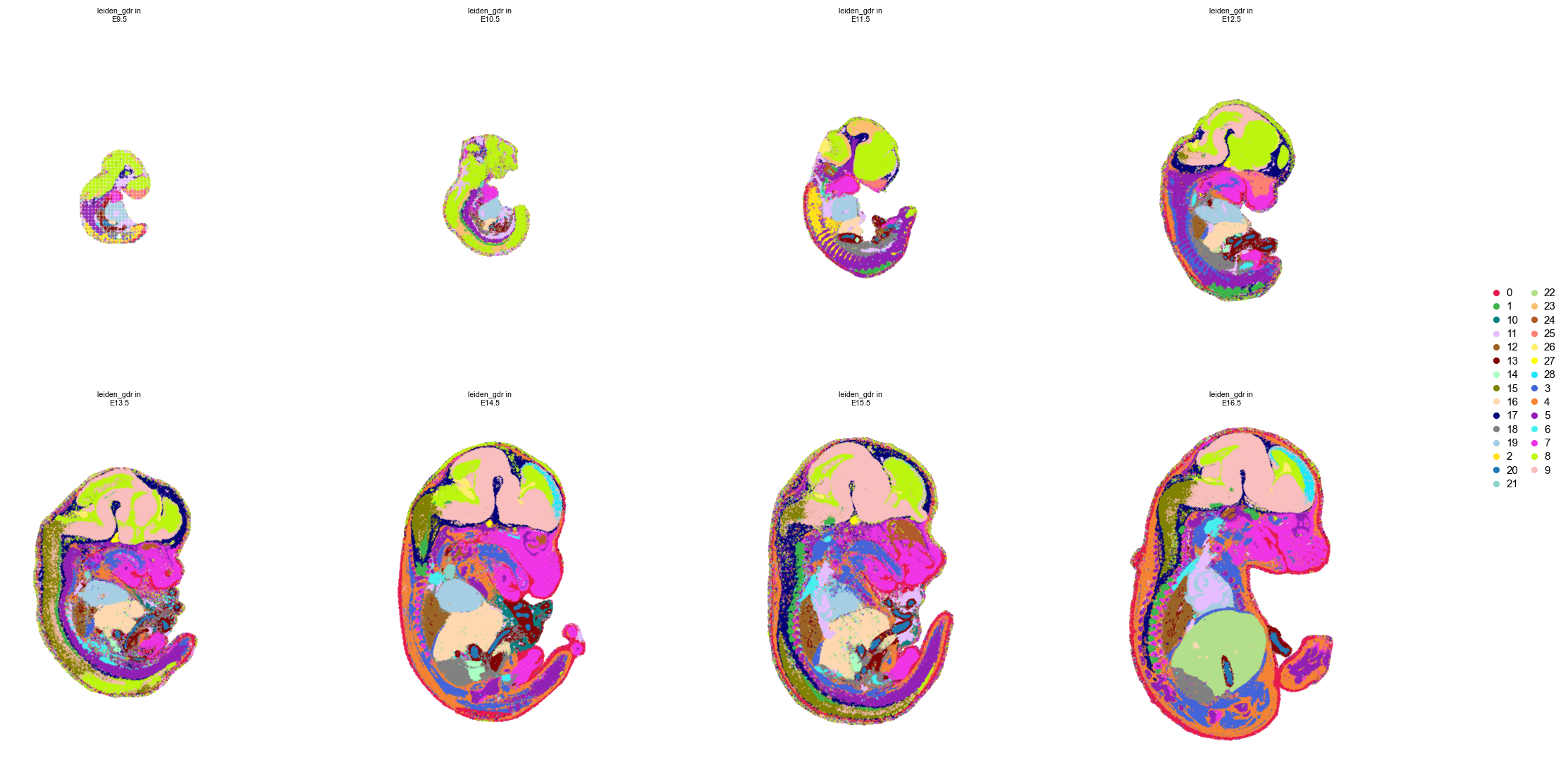

alignSpatialCoordinates is the step that makes that grid readable. Each section is placed on its own chip, so raw coordinates put the eight embryos hundreds of microns apart and the shared axes of a split plot stretch to cover the union — every panel ends up a small blob in a corner. Centring each sample on its own centroid fixes the framing and nothing else: it is a translation, so within-sample distances are untouched. Pass scale_units=True as well when sections come from different platforms or magnifications and only the shape is comparable — here they do not, and an E9.5 embryo really is smaller than an E16.5 one, so the sizes should differ.

4. Cost

Step	Wall clock	Notes
INFOG, 520,815 × 23,761	~400 s	streamed, ~1.5 GB RSS
`runGDR`, `batch_key="timepoint"`	~700 s	16 workers, writes `X_gdr` to disk
UMAP on 520,815 × 162	773 s	single-threaded — see below

The UMAP is the slowest step and the only one that holds everything in memory. random_state=1927 forces n_jobs=1, which umap-learn warns about: reproducibility costs you the parallel build. Drop the seed for a several-fold speedup when you do not need the run to be bit-reproducible, or subsample for a first look — the GDR embedding itself is already computed and does not change.

5. Notes

batch_key and groupby do different jobs. groupby defines the marker sets; batch_key decides within which groups those markers are found. Passing batch_key without groupby scores against markers of whatever clustering GDR runs itself.
Check both colourings, always. A single panel cannot distinguish integration from over-correction.
The embedding is on disk. runGDR writes X_gdr into the cytome and returns None, mirroring scanpy’s in-place convention. Re-opening the file is enough; nothing needs recomputing.