
cytorete across development: regulon dynamics at half a million bins
The spatial tutorial ran one Stereo-seq section. This runs all eight, from the full MOSTA series — E9.5 to E16.5, 520,815 bins × 23,761 genes, 45 annotated organs — in one pass, and asks a question a single section cannot: when is each regulon active?
Nothing here is a time-series method. inferRegulon is given organ labels
and never sees a stage. The developmental ordering falls out afterwards,
which is what makes it worth plotting.
1. One file, eight stages
import piasoimport cytome, piaso, cytorete, numpy as np
ds = cytome.open("mosta_all.cytome")ds.n_cells # 520815piaso.settings.set_figure_params(style="cell") # one house style across every figure| Stage | Bins | Stage | Bins | |
|---|---|---|---|---|
| E9.5 | 5,913 | E13.5 | 77,369 | |
| E10.5 | 18,408 | E14.5 | 102,519 | |
| E11.5 | 30,124 | E15.5 | 113,350 | |
| E12.5 | 51,365 | E16.5 | 121,767 |
INFOG from the raw layer, then regulons — the same two calls as on one section, with no change for the twentyfold increase in bins:
piaso.tl.infog(ds, modality="RNA", layer="count",               key_added="infog", save_layer=True, inplace=True)ds.flush(); ds.close()
TFS = ["Sox2", "Pax6", "Sox10", "Foxa2", "Hnf4a", "Myod1", "Myog", "Gata4",       "Twist1", "Cdx2", "Olig1", "Lhx2", "Emx2", "Tbx5", "Neurod1", "Ascl1",       "Gata1", "Tal1", "Runx1", "Hand2", "Nkx2-5", "Pdx1", "Six1",       "Pou3f2", "Rfx4"]
cytorete.inferRegulon("mosta_all.cytome", "mm10", "annotation",                      jaspar_path=piaso.data.fetch_jaspar(),                      twobit_path=piaso.data.fetch_2bit("mm10"),                      tf_list=TFS, cosg_layer="infog", score_layer="infog")
[inferRegulon] 24 TFs with motifs in the data[inferRegulon] 4079 genes with promoters (6414 intervals)[cistrome] M = 24 TFs × 4079 genes, 10324 edges (10.55% density)cospecificity_trans: 3182 positive-sign edges over 45 cell types[regulons] 20 global regulons (median 135 targets); per-cell-type for 32Scalability
| Step | Wall clock | Peak RSS |
|---|---|---|
| INFOG, 520,815 × 23,761 | 397 s | ~1.5 GB |
inferRegulon (incl. COSG, cistrome, activity) | 178 s | ~1.5 GB |
| Total | 575 s |
Under ten minutes for half a million bins on one machine, at a memory footprint that does not depend on the number of bins — the matrix is streamed in chunks and never held whole. The COSG pass inside it reports its own timing: 255 chunks, 520,815 cells, 14.4 s of compute.
2. When each regulon peaks
Activity is per bin. Averaging within stage gives a regulon × stage matrix; z-scoring each row and sorting by the stage of the maximum turns it into a wave:
import json, pandas as pd
ds = cytome.open("mosta_all.cytome")md = ds.metadata["regulon"]md = json.loads(md) if isinstance(md, str) else mdnames = md["names"]A = np.asarray(ds.embeddings["X_regulon"])assert A.shape[1] == len(names)          # never index by your TF list
stage = np.asarray(ds.cells["timepoint"]).astype(str)ORDER = ["E9.5","E10.5","E11.5","E12.5","E13.5","E14.5","E15.5","E16.5"]M = pd.DataFrame({n: pd.Series(A[:, j]).groupby(stage).mean()                  for j, n in enumerate(names)}).T[ORDER]Z = M.sub(M.mean(axis=1), axis=0).div(M.std(axis=1), axis=0)
Order the stages once, on the file, so every later plot and groupby follows
the developmental sequence instead of alphabetical order (E10.5 before
E9.5):
ORDER = ["E9.5","E10.5","E11.5","E12.5","E13.5","E14.5","E15.5","E16.5"]ds.set_categories("timepoint", ORDER) # stored in the cytomeThen the figure — both panels, so it reproduces exactly:
import matplotlib.pyplot as plt
Z = Z.iloc[np.argsort(Z.values.argmax(axis=1))]     # rows by peak stagedelta = (M[ORDER[-3:]].mean(axis=1) - M[ORDER[:3]].mean(axis=1)).sort_values()
fig, (ax1, ax2) = plt.subplots(1, 2, figsize=(15, 6),                               gridspec_kw={"width_ratios": [1.2, 1]})im = ax1.imshow(Z.values, aspect="auto", cmap="RdBu_r", vmin=-2, vmax=2)ax1.set_xticks(range(8)); ax1.set_xticklabels(ORDER, rotation=45, ha="right")ax1.set_yticks(range(len(Z))); ax1.set_yticklabels(Z.index, fontsize=9)ax1.set_title("regulon activity across development\n(row z-score, ordered by peak stage)")fig.colorbar(im, ax=ax1, fraction=0.03)
SHOW = list(delta.index[:3]) + list(delta.index[-3:])       # 3 down, 3 upfor n, c in zip(SHOW, ["#4E79A7","#56B4E9","#7D80DA","#E69F00","#D55E00","#CC79A7"]):    ax2.plot(range(8), M.loc[n].values, marker="o", ms=5, lw=2, color=c, label=n)ax2.set_xticks(range(8)); ax2.set_xticklabels(ORDER, rotation=45, ha="right")ax2.set_ylabel("mean regulon activity")ax2.set_title("the three that fall and the three that rise")ax2.legend(frameon=False, fontsize=10, ncol=2)ax2.spines[["top","right"]].set_visible(False)fig.tight_layout()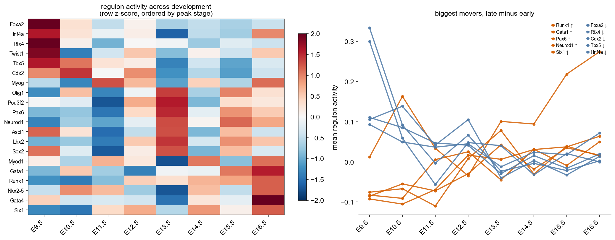
The rows sort themselves into three blocks, and each is right:
| Peaks at | Regulons | What that is |
|---|---|---|
| E9.5 | Foxa2, Hnf4a, Rfx4, Twist1, Tbx5 | definitive endoderm, early mesenchyme, early cardiac |
| E10.5–11.5 | Cdx2, Myog | posterior/gut patterning, first myogenesis |
| E13.5 | Sox2, Pax6, Ascl1, Neurod1, Olig1, Pou3f2, Lhx2 | the entire neurogenic set, together — peak neurogenesis |
| E16.5 | Gata1, Runx1, Gata4, Nkx2-5, Myod1, Six1 | definitive haematopoiesis, cardiac and muscle maturation |
That seven neural TFs independently peak at the same stage, with no shared targets forced and no temporal term in the model, is the result worth pausing on. Ranking by late-minus-early activity says the same:
falls: Foxa2 −0.149 Rfx4 −0.105 Cdx2 −0.101rises: Pax6 +0.092 Gata1 +0.126 Runx1 +0.133Gata1 and Runx1 climbing hardest across E13.5→E16.5 is the switch to definitive haematopoiesis in the fetal liver, which those bins are full of.
2b. The same regulon, section by section
The heatmap says when. The sections say where, and put the two together:
piaso.pp.rotateSpatialCoordinates(ds, angle_degrees=90, spatial_key="spatial")piaso.pp.alignSpatialCoordinates(ds, batch_key="timepoint",                                 spatial_key="spatial",                                 key_added="spatial_aligned")
# a shared range across panels, tight enough that the signal is not# flattened by a long upper tailv = np.asarray(ds.cells["regulon_Sox2"], dtype=float)lo, hi = np.percentile(v, [40, 99.5])
piaso.pl.plot_embeddings_split(ds, color="regulon_Sox2", splitby="timepoint",                               basis="spatial_aligned", ncols=4,                               cmap="Spectral_r", vmin=lo, vmax=hi)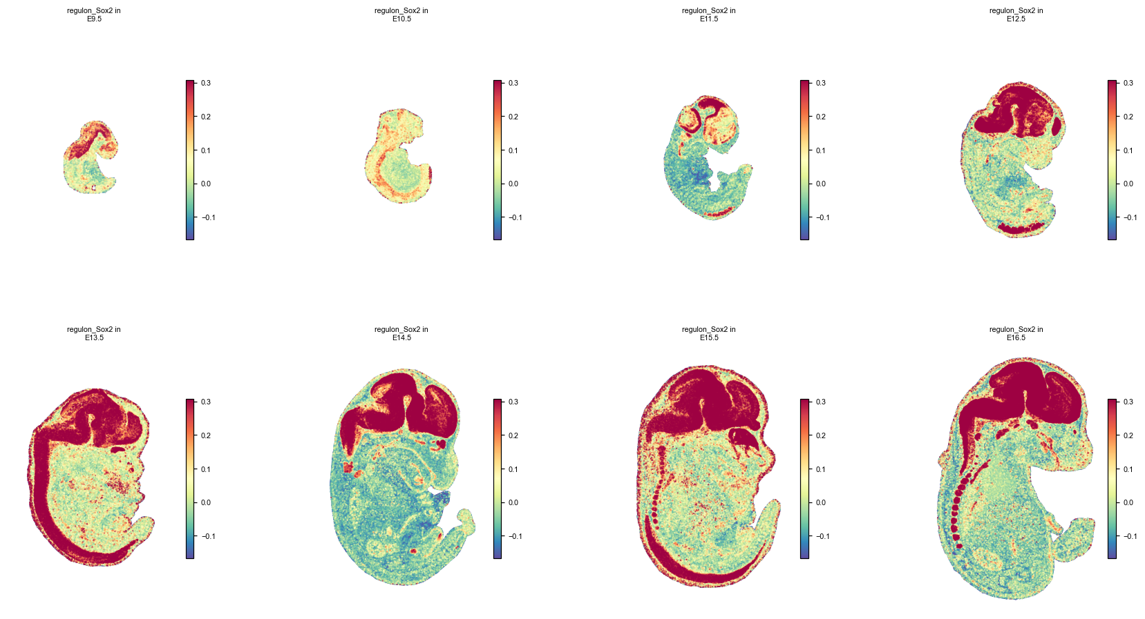
vmin/vmax rather than vmin_pct/vmax_pct here on purpose: a split plot
shares one colour range across every panel, so the range has to be chosen
from the whole series. Sox2 runs from −1.46 to 2.81 with most bins near zero,
and on the full range every panel is one shade of green.
Alignment matters here: the eight sections sit at different chip offsets, so without centring each stage on its own centroid the panels render at different positions and the series is unreadable.
Sox2 marks the neural tube at E9.5 — nearly the whole embryo at that stage — and then contracts onto brain and spinal cord as everything else differentiates around it. The heatmap’s E13.5 peak and this contraction are the same fact seen twice.
The organ labels, drawn the same way, are the control:
piaso.pl.plot_embeddings_split(ds, color="annotation", splitby="timepoint", basis="spatial_aligned", ncols=4)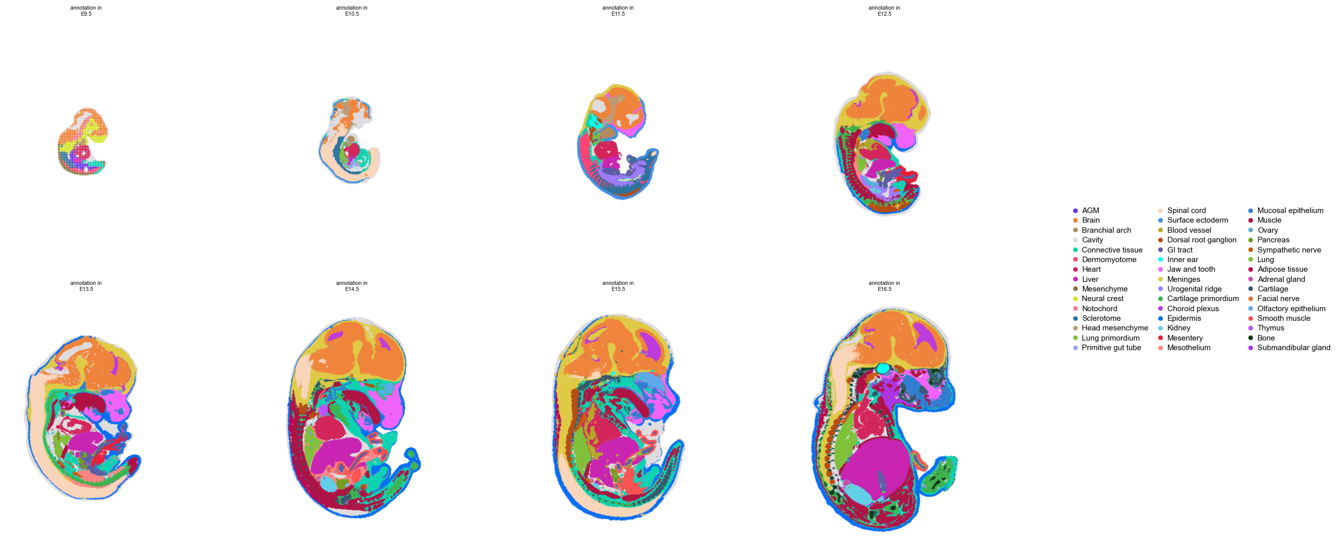
Compare the two: where a regulon’s activity tracks an organ that is itself appearing over the series, the regulon is following tissue composition; where it moves within an organ that is present throughout, it is telling you something the annotation does not.
3. What more groups buy you
On the single E16.5 section, Lhx2 produced zero co-specificity edges
and no regulon. Here it has one.
The tempting explanation is a finer annotation — but check before believing
it: E16.5 alone still carries 25 labels here, and the brain is still one
Brain label. The 45 categories come from pooling stages, because
different stages contribute different organs. So the anatomy did not get
finer; the grouping got wider.
That is the real lever. Co-specificity asks whether a TF and a candidate
target covary across groups. Adding seven more stages adds groups spanning
developmental states — early neuroepithelium is a different context from
late brain even when both are labelled Brain — and Lhx2’s targets now
have something to vary against.
Sox10 and Emx2 are still absent, so this is not a cure-all. Both remain
restricted within one label at every stage. Sub-annotating the brain is the
untested prediction; widening across stages is the one this tutorial
actually demonstrates.
4. Notes
- Composition changes with stage, so read a rise carefully. Later embryos
have both more bins and different organs. Averaging over the whole embryo
mixes “this regulon got more active per cell” with “its tissue grew” —
Gata1’s climb is partly the fetal liver becoming a larger share of the section. To separate them, average within one annotation across stages instead of over everything. assert A.shape[1] == len(names). Five of the 25 TFs dropped; a positional index built from your input list would be silently wrong.- Per-cell-type regulons exist for 32 of 45 organs (
md["per_celltype"]) — the same TF carries different targets in liver than in brain. - Stage is not a covariate here. If you want stage-aware regulons rather
than stage-resolved activity, pass
groupbya column that crosses organ with stage.