
COSG on a cytome
Everything in chapter 1 assumed the expression
matrix was in memory. run_cosg_cytome does the same analysis by streaming the
matrix in chunks off disk, so memory is set by the chunk size rather than by
the number of cells.
1. Open the file
The same cortex dataset as chapter 1, as a cytome.
import cytome, cosg, piaso
ds = piaso.data.load_dataset("adult_cortex_multiome_rna", return_type="cytome")ds.n_cells, [c for c in ds.cells.columns if "CellTypes" in c]
(17412, ['CellTypes_TACCO', 'CellTypes'])return_type="cytome" converts the cached download once and reopens it on
later calls; cytome.open("adult_cortex_multiome_rna.cytome") does the same
thing when you already have the file.
The embeddings travel with the file, so you can look at it before scoring
anything — piaso.pl.embedding takes the Dataset directly, no AnnData in
between:
piaso.pl.embedding(ds, color="CellTypes", basis="X_umap", legend_loc="on_data", legend_fontsize=6)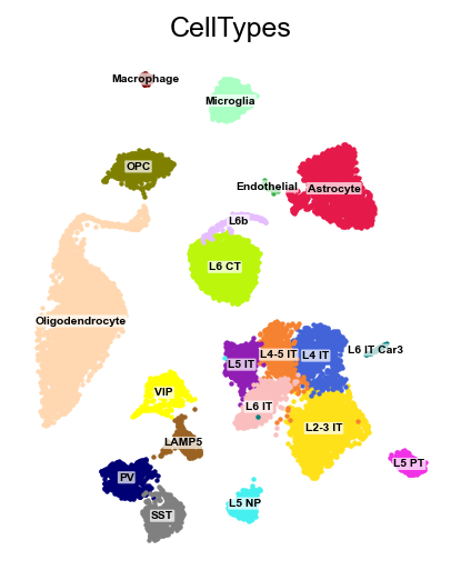
2. Run COSG
res = cosg.run_cosg_cytome( ds, groupby="CellTypes", # a column in the cells table layer="auto", # normalise the stored raw counts on the fly mu=100, n_genes_user=50, calculate_pvalues=True, output_format="ndarray",)sorted(res.keys())['groups_order', 'names', 'pvals', 'pvals_adj', 'scores']Fourteen seconds for 17,412 cells × 26,205 genes. The result is arrays rather
than an adata.uns entry, because there is no AnnData:
import pandas as pdmarkers = pd.DataFrame(res["names"], columns=list(res["groups_order"]))markers.head(3) L2-3 IT L4 IT L4-5 IT L5 IT0 Otof Rspo1 Scn7a Deptor1 Ccbe1 Gm40331 Tnnc1 Il1rapl22 Evc2 Gm42953 BC006965 Rxfp2output_format controls the shape, and this is where the streaming path
differs most from the in-memory one — there is no adata.uns to write into, so
the result is returned:
output_format | what you get |
|---|---|
"ndarray" (used above) | names and scores as (n_genes_user, n_groups) arrays, plus groups_order; the closest analogue of adata.uns['cosg'] |
"dict" | scores_dict keyed by (group, gene), with groups_order and group_sizes — convenient for lookups |
"dense" | a full feature × group DataFrame indexed by every feature in the file, missing entries 0; the analogue of indexByGene output, and the one to pass to iqrLogNormalize |
"long" | one row per (group, gene, score) |
calculate_pvalues=True adds pvals and pvals_adj to whichever shape you
chose. For the cross-cell-type comparison described in
chapter 1,
ask for "dense" with n_genes_user set to the full feature count and hand
the result straight to cosg.iqrLogNormalize — no indexByGene step, because
the dense form is already genes × groups.
The markers, on the file’s own embedding
Reading a marker back out needs nothing but the gene name — the plot function resolves it against the cytome’s feature table and streams the column:
genes = [markers[c][0] for c in ("Oligodendrocyte", "Astrocyte", "Microglia", "L2-3 IT")]piaso.pl.embedding(ds, color=genes, basis="X_umap", layer="log1p", ncols=4)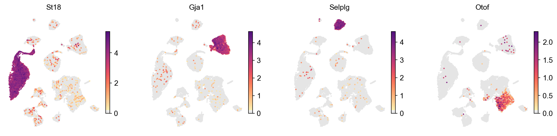
St18, Gja1, Selplg and Otof — the canonical oligodendrocyte, astrocyte,
microglial and L2-3 markers. Note layer="log1p" here rather than "auto":
auto is a COSG argument meaning “normalise the raw counts as you stream”, and
the plot function wants the name of a layer it can compute, so asking it for
"auto" raises with the list of layers it does know.
3. What layer= means here
This is the one parameter that behaves differently from the in-memory call.
A cytome stores named matrices, and layer chooses which one COSG reads:
layer="auto"(default) takes the raw counts and normalises each chunk as it streams — the usual choice when the file holdsRNA_counts.layer="data"or any stored name reads that matrix as-is. Use this when the file already holds a normalised matrix, or when you want to control the normalisation yourself.
4. Significance, streamed
calculate_pvalues=True works the same way and means the same thing as in
chapter 1 —
including that the labels must not have come from clustering this same matrix.
The implementation differs in a way worth knowing if you are comparing backends. The moments COSG needs are power sums, which add across chunks, so they come from the pass that computes the cosine anyway. The tail refinement needs each flagged gene’s value distribution, which is accumulated over a second pass as a fixed-grid histogram — also additive. The streamed summary is identical to the in-memory one, not merely close, so the two paths return the same p-values rather than agreeing to some tolerance.
One limitation: batch_key with
calculate_pvalues=True raises on the streaming path. The stratified null needs per-batch power sums that the current
pass does not accumulate, and refusing is better than silently computing an
unstratified null. Batched significance runs work in memory.
You own the Dataset, so close it when you are done:
ds.close()5. When to use which
in-memory cosg.cosg | run_cosg_cytome | |
|---|---|---|
| input | AnnData | cytome file or open Dataset |
| memory | the whole matrix | one chunk |
| result | adata.uns[key_added] | returned arrays |
batch_key + p-values | yes | raises |
Below a few hundred thousand cells with the object already loaded, the in-memory call is simpler. Above that, or when the matrix does not fit, or when the file is the thing you keep, the streaming path is the one that scales — see GDR at scale for the same argument on embeddings.
Where to go next
- Batches —
batch_key, and which markers survive it. - COSG on the GPU — the other axis of scale.
- COSG on spatial data — a cytome with 121,767 spatial bins.
- cytome basics — what else the file holds.