Atera WTA: near-whole-transcriptome in situ

Every targeted spatial platform starts with the same problem: you have to choose the genes before you see the tissue. A 313-plex breast panel is excellent at the biology it was designed for and blind to everything else, and you find out which is which after the run.

10x’s Atera removes the choice — 18,028 targets in situ. This page runs the public FFPE human breast cancer section from its WTA preview: 170,057 cells × 18,028 genes, and then asks the question the technology exists to answer — what would a panel have missed?

Atera is a different platform from Xenium, not a Xenium panel: the run’s own metadata reports chemistry_version: Atera v1 on an Insitu Gen2 Prototype Instrument. What it shares with Xenium is the output format — the same cell_feature_matrix.h5, cells.parquet, morphology_focus/ bundle, and an analysis pipeline still versioned xenium-* — which is why every loading and plotting call below is identical to the Xenium pages, and why the two can be compared directly.

How “whole” is whole?

WTA stands for Whole Transcriptome Analysis, which is the product name rather than a measurement. Against GENCODE v44 it is worth being exact:

# 18,028 targets, against the annotation
protein_coding = 20,020         # unique gene names in GENCODE v44
targets & protein_coding        # 18,013  -> 90.0% of protein-coding genes
targets - protein_coding        #     15  -> almost nothing else
all_annotated_genes = 62,700    # 18,028  -> 28.8% of everything

So: 90% of the protein-coding transcriptome, and 29% of the annotated transcriptome. All but 15 of its targets are protein-coding, which means essentially no lncRNA (18,866 in the annotation), no pseudogenes and no small RNAs. If your question involves a non-coding transcript, this panel does not have it, and “whole transcriptome” would have told you otherwise.

Near-whole-transcriptome is the honest description, and 90% of coding genes is still a different kind of experiment from a 313-plex.

Spatial — Xenium and Atera

Xenium Prime 5K on mouse brain is the same workflow step by step, on a tissue whose anatomy is known — read that one first if you want the pipeline explained · Xenium with tissue-image overlay · Xenium into a cytome

1. The data

The full bundle is 55.2 GB. The parts an analysis needs are under 500 MB, and they can be pulled out of the remote ZIP without downloading the rest — the range-request reader is in the mouse brain tutorial, and only the URL changes:

URL = ("https://s3-us-west-2.amazonaws.com/10x.files/samples/atera/dev/"
       "WTA_Preview_FFPE_Breast_Cancer/WTA_Preview_FFPE_Breast_Cancer_outs.zip")

for name in ("experiment.xenium", "cells.parquet",
             "cell_feature_matrix.h5", "analysis.tar.gz"):
    ...

cell_feature_matrix.h5 is 398 MB here rather than 54 MB, which is the first sign of what has changed.

import json
meta = json.load(open("experiment.xenium"))
meta["panel_name"], meta["panel_num_targets_predesigned"], meta["num_cells"]

('Human WTA (pre-release)', 18028, 170057)

Loading is identical to a Xenium run, because the output bundle is the same:

import numpy as np
import pandas as pd
import piaso, cosg

adata = piaso.pp.read_10x_h5("cell_feature_matrix.h5")
adata.var_names_make_unique()

cells = pd.read_parquet("cells.parquet")
cells["cell_id"] = cells["cell_id"].astype(str)
cells = cells.set_index("cell_id").loc[adata.obs_names]
adata.obsm["spatial"] = cells[["x_centroid", "y_centroid"]].to_numpy()
for col in ("transcript_counts", "control_probe_counts",
            "control_codeword_counts", "cell_area"):
    adata.obs[col] = cells[col].values

adata.shape, np.median(adata.obs["transcript_counts"])

((170057, 18028), 2116.0)

2,116 transcripts per cell at the median, across 18,028 targets. For comparison the 5K mouse brain run gives 1,088 across 5,006. More targets and more counts per cell.

2. Is it really measuring 18,000 genes?

This is the first thing to check, and the honest answer is a curve rather than a yes.

adata = adata[(adata.obs["transcript_counts"] >= 25)
              & (adata.obs["cell_area"] > 0)].copy()
adata.layers["counts"] = adata.X.copy()

cells_per_gene = np.asarray((adata.layers["counts"] > 0).sum(axis=0)).ravel()
(cells_per_gene > 0.01 * adata.n_obs).sum(), (cells_per_gene == 0).sum()

(16303, 0)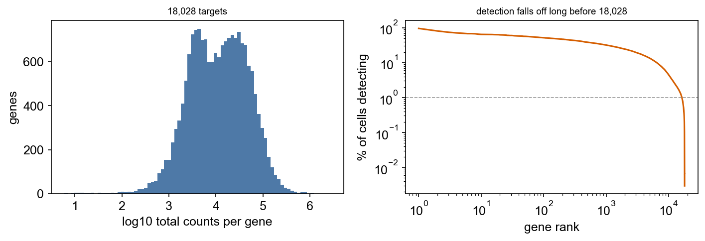

• No gene is never detected. All 18,028 targets produce signal somewhere.
• 16,303 of 18,028 (90%) are detected in more than 1% of cells.
• The median gene is seen in 9,740 cells.

So the claim holds up better than “whole transcriptome” claims usually do. The right-hand panel is still the one to remember: detection falls off steeply, and the bottom couple of thousand genes are present but too sparse to cluster on. That is a floor, not a failure — the same curve exists in scRNA-seq, where it is rarely drawn.

The negative controls give the background as before:

ctrl = adata.obs["control_probe_counts"] + adata.obs["control_codeword_counts"]
100 * ctrl.sum() / (adata.obs["transcript_counts"] + ctrl).sum()

0.017

0.017% — higher than the mouse brain run’s 0.007%, still negligible. Worth noting that a whole-transcriptome panel has more opportunity for cross-hybridisation, and the control rate is how you would see it if it happened.

3. Clusters and markers

Unchanged from any other dataset. Nothing in the pipeline knows this is spatial, or that it is 18,000-plex.

# INFOG, then a preliminary grouping, then GDR as the actual embedding
piaso.tl.infog(adata, layer="counts", n_top_genes=3000, key_added="infog")
piaso.tl.runSVD(adata, layer="infog", n_components=50, key_added="X_svd",
                scale_data=False)
piaso.tl.neighbors(adata, use_rep="X_svd", n_neighbors=15)
piaso.tl.leiden(adata, resolution=1.0, key_added="leiden_prelim")

piaso.tl.runGDR(adata, groupby="leiden_prelim", layer="infog",
                score_layer="infog", n_gene=30, mu=10.0)
piaso.tl.neighbors(adata, use_rep="X_gdr", n_neighbors=15)
piaso.tl.leiden(adata, resolution=1.0, key_added="leiden")
piaso.tl.umap(adata, use_rep="X_gdr")

adata.X = adata.layers["infog"]
cosg.cosg(adata, groupby="leiden", key_added="cosg", mu=100, n_genes_user=30,
          calculate_pvalues=True)

The dimensionality reduction is INFOG + GDR, exactly as in the mouse brain page — the SVD only exists to give GDR a preliminary grouping to build axes on. The interesting difference is that with 18,028 genes the SVD has far more to work with than on a panel, and GDR still changes the answer, because “explains variance” and “distinguishes cell identity” are different objectives however many genes you have.

The marker lists are where the extra genes start to show:

cluster	top markers	reading
3	TRAC, CD3E, ZAP70, TRBC2, TRBC1	T cells
1	IGHG1, PDK1, IGKC, TENT5C, CD79A	plasma / B cells
4	C7, THBS2, FGF7, TNXB, SRPX	fibroblasts
6	PLVAP, VWF, SLCO2A1, AQP1	vascular endothelium
7	GJA5, SEMA3G, VEGFC, MECOM	arterial endothelium
5	MMRN1, PROX1, PKHD1L1, CCL21	lymphatic endothelium
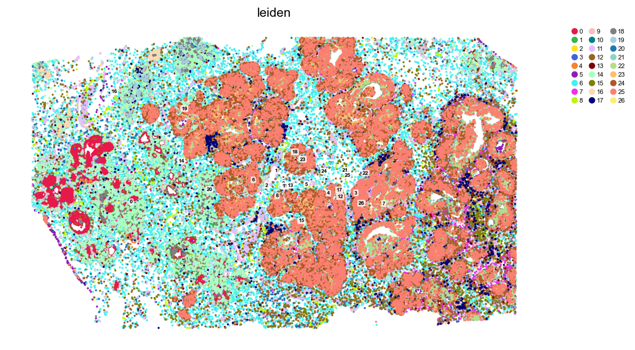
0	CACNG4, BMPR1B, SLC24A3, NIBAN1	tumour epithelium

Three separate endothelial identities — general vascular, arterial and lymphatic — resolved as distinct clusters and named by genes (GJA5, MMRN1, CCL21) that no breast cancer panel would spend targets on.

The top three markers of every cluster in one panel — the check that each cluster has something of its own:

names = pd.DataFrame(adata.uns["cosg"]["names"])
feats = list(dict.fromkeys(g for c in names.columns for g in names[c][:3]))

adata.X = adata.layers["log1p"]
piaso.pl.dotplot(adata, features=feats, groupby="leiden",
                 swap_axes=True, cmap="Spectral_r",
                 standard_scale="var")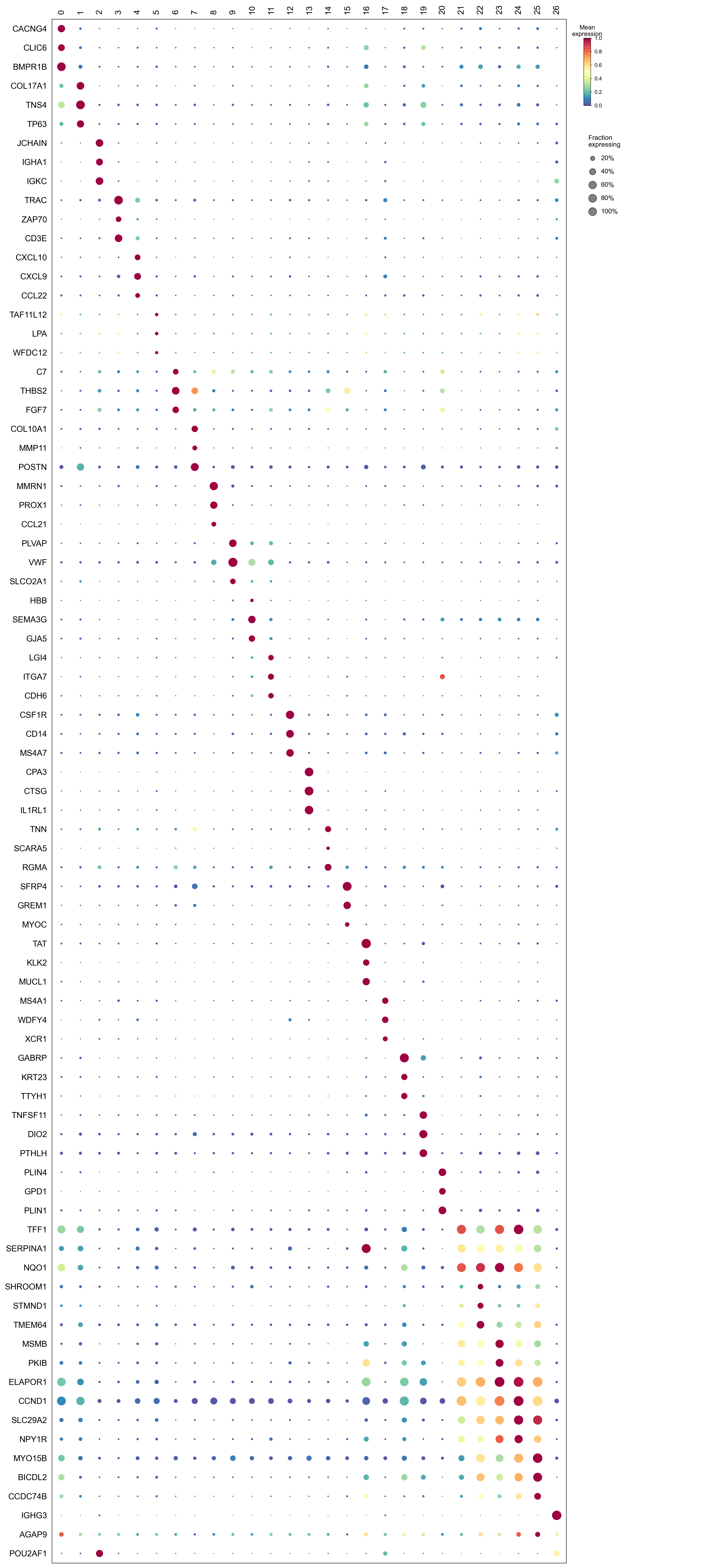

standard_scale="var" scales each gene to [0, 1] across clusters, so an abundant gene does not colour its whole column dark and drown the contrast that matters. The diagonal is what you want to see. Note piaso.pl.dotplot writes its own file — pass save= rather than calling plt.savefig afterwards, because it closes the figure when show=False.

3a. Are the big luminal clusters low quality?

Five clusters — 21 to 25 — all come back lumhr, which looks like a failure worth investigating before going further. The instinct is that they are low-quality cells that clustered together on noise. Check it before acting on it, because dropping them would remove 40% of the section.

piaso.pl.plotFeaturesViolin(
    adata, ["transcript_counts", "cell_area", "nucleus_area"],
    groupby="leiden", ncol=1, height_single=2.4)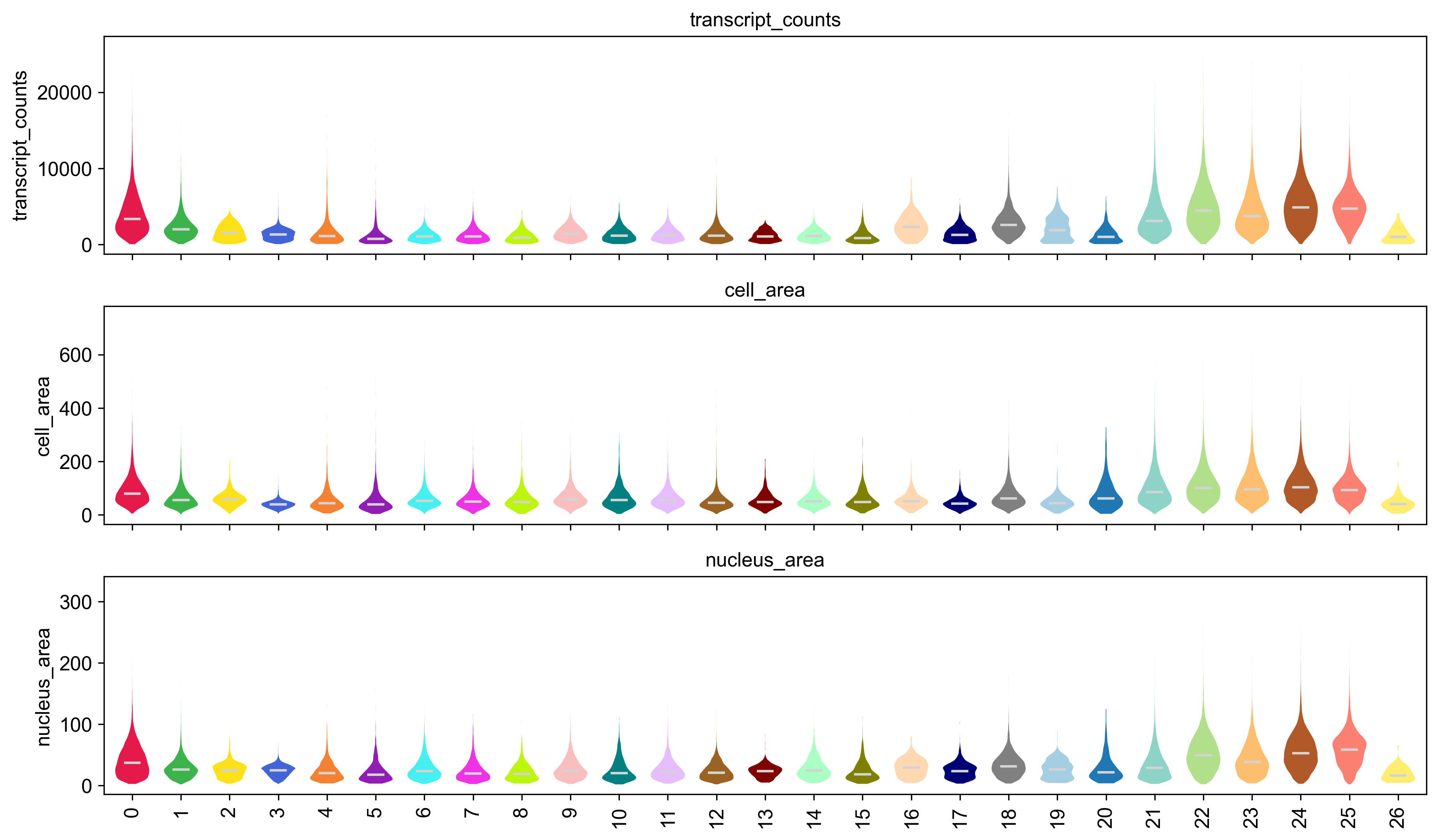

The answer is the opposite of the hypothesis:

	clusters 21–25	everything else
cells	68,426 (40.3%)	101,489
median transcripts	4,146	1,428
cell area	largest in the section	—
negative-control rate	0.019%	0.02%

They have the most signal, not the least — nearly three times the transcripts of the rest of the section, the largest cells and nuclei, and a background rate identical to everything else. Low-quality cells look like the opposite of this: few transcripts, small area, elevated controls.

Their markers say what they are:

cluster	top markers
21	TFF1, SERPINA1, NQO1, BRMS1
22	SHROOM1, STMND1, TMEM64, ALDH3B2
23	MSMB, PKIB, ELAPOR1, TFF3
24	CCND1, SLC29A2, NPY1R, MYEOV
25	MYO15B, BICDL2, CCDC74B, PLIN5

These are malignant epithelium, and heterogeneous within itself. TFF1 and TFF3 are oestrogen-regulated trefoil factors; CCND1 and MYEOV are the two genes of the 11q13 amplicon, one of the commonest amplifications in breast cancer, appearing together in the same cluster.

So the five clusters are not one cell type badly split — they are the tumour, which is genuinely several transcriptional states. What produced the appearance of failure was the reference: Kumar/Navin is a normal breast atlas with a single lumhr category, so five malignant states collapse onto one normal label. That is the same lesson as §4 below, reached from the other direction.

Could they be doublets?

Worth asking, because high counts and large area are also the classic doublet signature — the argument above would run identically for cells that are two cells merged by segmentation. The output bundle gives three ways to check, and all three say no.

Its own multi-nucleus flag. cells.parquet carries nucleus_count, so a merged cell that caught both nuclei is directly visible:

mn = adata.obs.groupby("leiden")["nucleus_count"].apply(lambda s: 100*(s > 1).mean())

	% of cells with > 1 nucleus
clusters 21–25	0.71%
all other clusters	0.53%
section-wide	0.54%

Not enriched, and the four most multi-nucleate clusters (19, 16, 26, 18) are not among them.

Lineage co-expression. A doublet of two different cell types carries both programmes, so count cells positive for two lineages that should be mutually exclusive:

lin = pd.DataFrame({
    "epi":  pos(["EPCAM", "KRT8", "KRT18"]),
    "imm":  pos(["PTPRC", "CD3E", "CD14", "MS4A1"]),
    "fib":  pos(["COL1A1", "COL1A2", "DCN"]),
    "endo": pos(["PECAM1", "VWF", "CLDN5"])})
(lin.sum(1) >= 2).groupby(adata.obs["leiden"]).mean() * 100

	% of cells positive for ≥ 2 lineages
clusters 21–25	3.7%
all other clusters	5.4%

They are less lineage-mixed than the rest of the section, not more. The mixed clusters are 12 (15.9%), 9 (11.1%) and 3 (9.7%) — the myeloid, endothelial and T-cell populations, which are exactly the small cells that sit wedged among everything else and are hardest to segment cleanly.

Arithmetic. These five clusters are 40.3% of the section. If they were doublets, the doublet rate would have to be 40%, which no segmentation produces.

None of this rules out the occasional merged pair of two epithelial cells, which would not show as lineage mixing — but that would be a small correction to a real population, not an explanation for it.

They stay in. Removing them would delete the tumour from a tumour analysis.

The tumour markers in tissue space

The last check is where these genes actually are:

piaso.pl.embedding(adata, color=["TFF1", "SERPINA1", "MSMB", "TFF3",
                                 "CCND1", "MYEOV"],
                   basis="spatial", point_size=0.45, ncols=3,
                   vmin_pct=2, vmax_pct=98, fix_coordinate_ratio=True)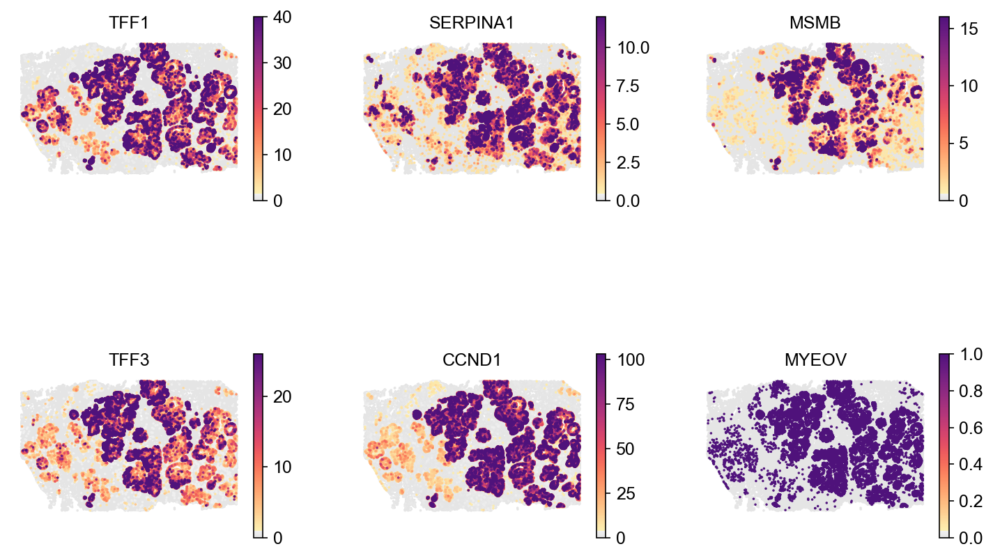

They fill the epithelial nests and stop at their edges — a spatially coherent compartment, not cells scattered through the section as a technical artefact would be. CCND1 is the clearest: detected in 64% of cells at a mean of 36 counts inside the tumour clusters against 2.6 outside, a 14-fold enrichment that draws the nests unambiguously.

MYEOV is the panel worth pausing on, because it shows a limit rather than a result. It is enriched in the same cells (0.22 counts against 0.02, 11-fold), but it is detected in only 7.8% of cells at all, so the percentile clipping collapses its colour scale to 0–1 and the panel reads as a mask rather than an expression gradient. Its per-cell correlation with CCND1 is only 0.31 — not because the two are unrelated, but because one of them is too sparse to correlate with anything at single-cell resolution.

That is a real property of a near-whole-transcriptome panel: 18,028 targets span a very wide range of detection, and a gene can be genuinely and specifically enriched while still being too sparse to plot. Check the detection rate before reading a spatial panel as a gradient.

The general point

A cluster that a reference cannot name is not the same as a cluster that should not exist. Check the QC metrics, then the markers, and only then decide. Reaching for a filter first would have thrown away the most interesting 40% of this section.

3b. Naming the clusters from PIASOmarkerDB

Clusters are not cell types until something names them, and for breast tissue PIASOmarkerDB carries the Kumar/Navin 2023 human breast atlas (Nature) in three forms:

study	cell types	median markers on this panel (of 50)
KumarNavin2023Breast_scRNA	10	48
KumarNavin2023Breast_scRNA_fineAnno	58	46
KumarNavin2023Breast_snRNA	11	40

46–48 of 50 markers survive. That is the near-whole-transcriptome dividend stated a different way: a marker database transfers almost intact, where on the 5,006-gene mouse panel the median type kept 18 of 50.

df, marker_sets = piaso.tl.getMarkers(
    study="KumarNavin2023Breast_scRNA", as_dict=True)

panel = set(adata.var_names)
kept = {k: [g for g in v if g in panel] for k, v in marker_sets.items()}
kept = {k: v for k, v in kept.items() if len(v) >= 5}

piaso.tl.predictCellTypeByMarker(
    adata, marker_gene_set=kept, score_method="piaso", score_layer="infog",
    use_rep="X_gdr", smooth_prediction=True, k_nearest_neighbors=7,
    key_added="CellTypes_breast")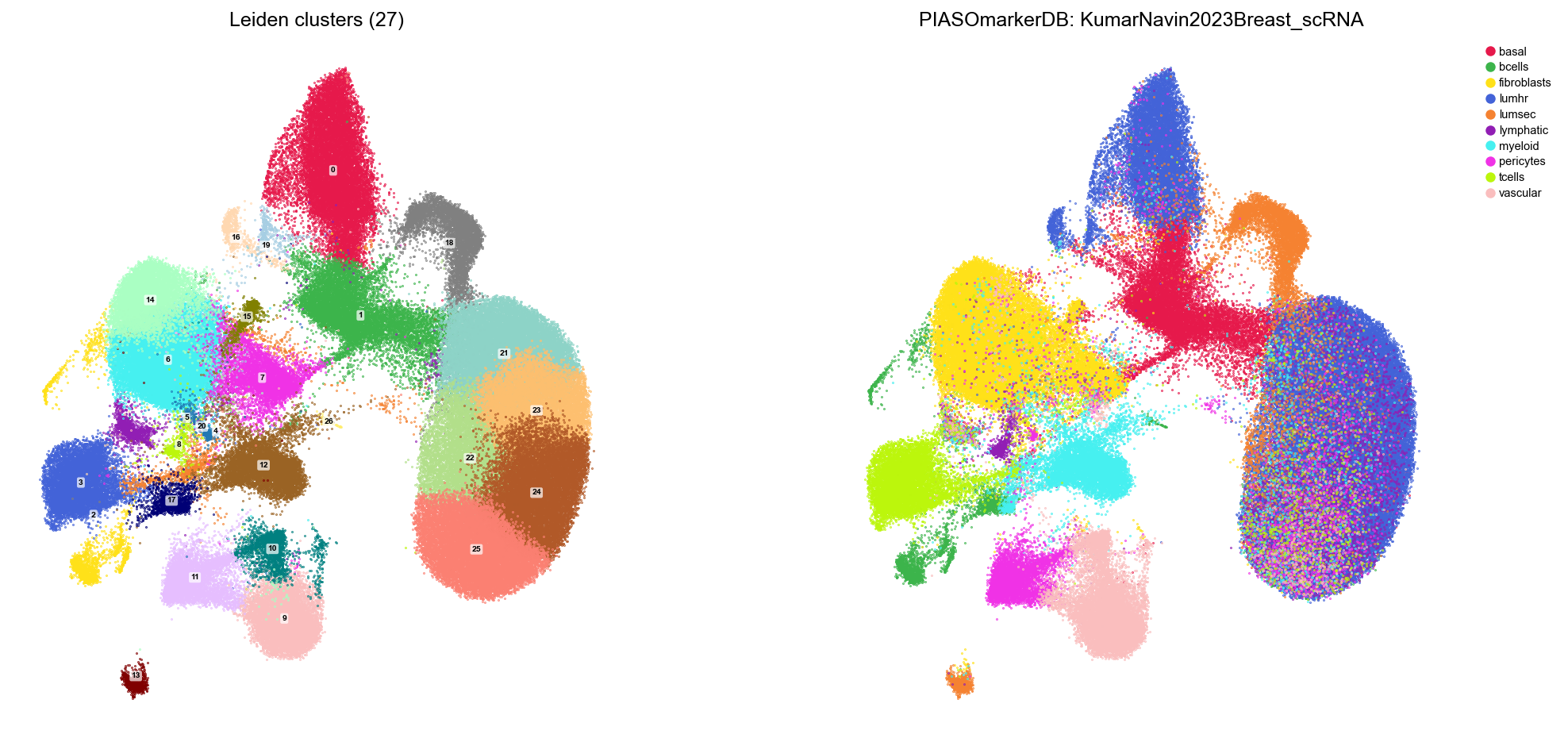

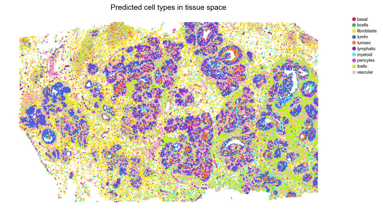
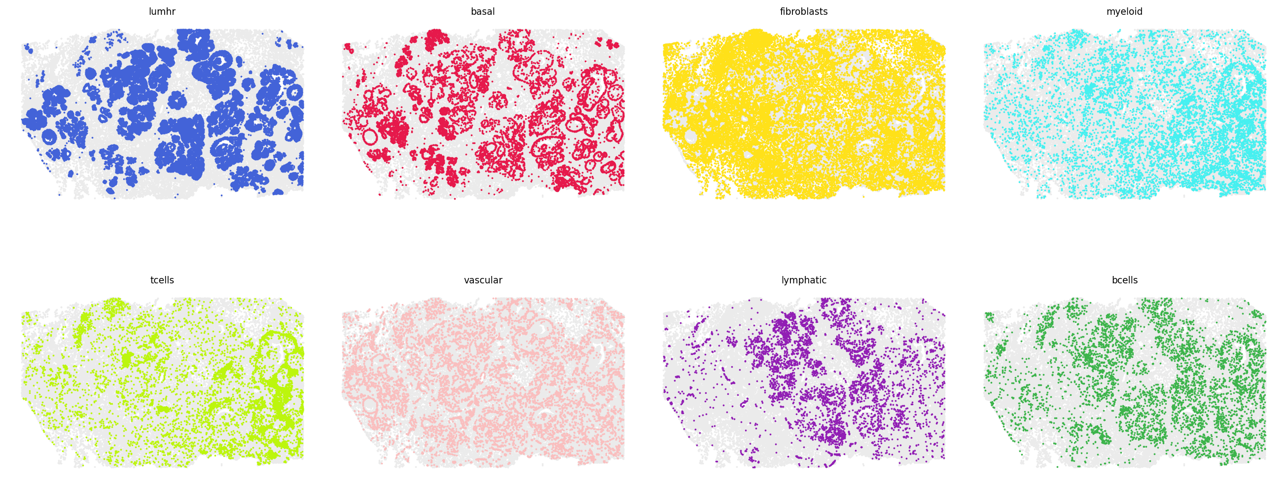
The tissue plot is where the labels stop being a list and become an anatomy. lumhr forms discrete epithelial nests; fibroblasts fill the stroma between them; vascular traces vessels through it; and tcells are not spread evenly but concentrated to one side of the section, which is the sort of observation that only exists because the coordinates were kept.

Does it agree with the clusters’ own markers?

The prediction never saw the COSG markers, so cross-tabulating the two is a real check:

cluster’s top markers	predicted	share of cluster
CSF1R, CD14, MS4A7, C1QC	myeloid	0.99
GABRP, KRT23, TTYH1, PROM1	lumsec	0.99
COL17A1, TNS4, TP63, OVCH2	basal	0.98
JCHAIN, IGHA1, IGKC, IGHA2	bcells	0.96
TNN, SCARA5, RGMA, LAMC3	fibroblasts	0.96
LGI4, ITGA7, CDH6, AVPR1A	pericytes	0.92
HBB, SEMA3G, GJA5, VEGFC	vascular	0.88

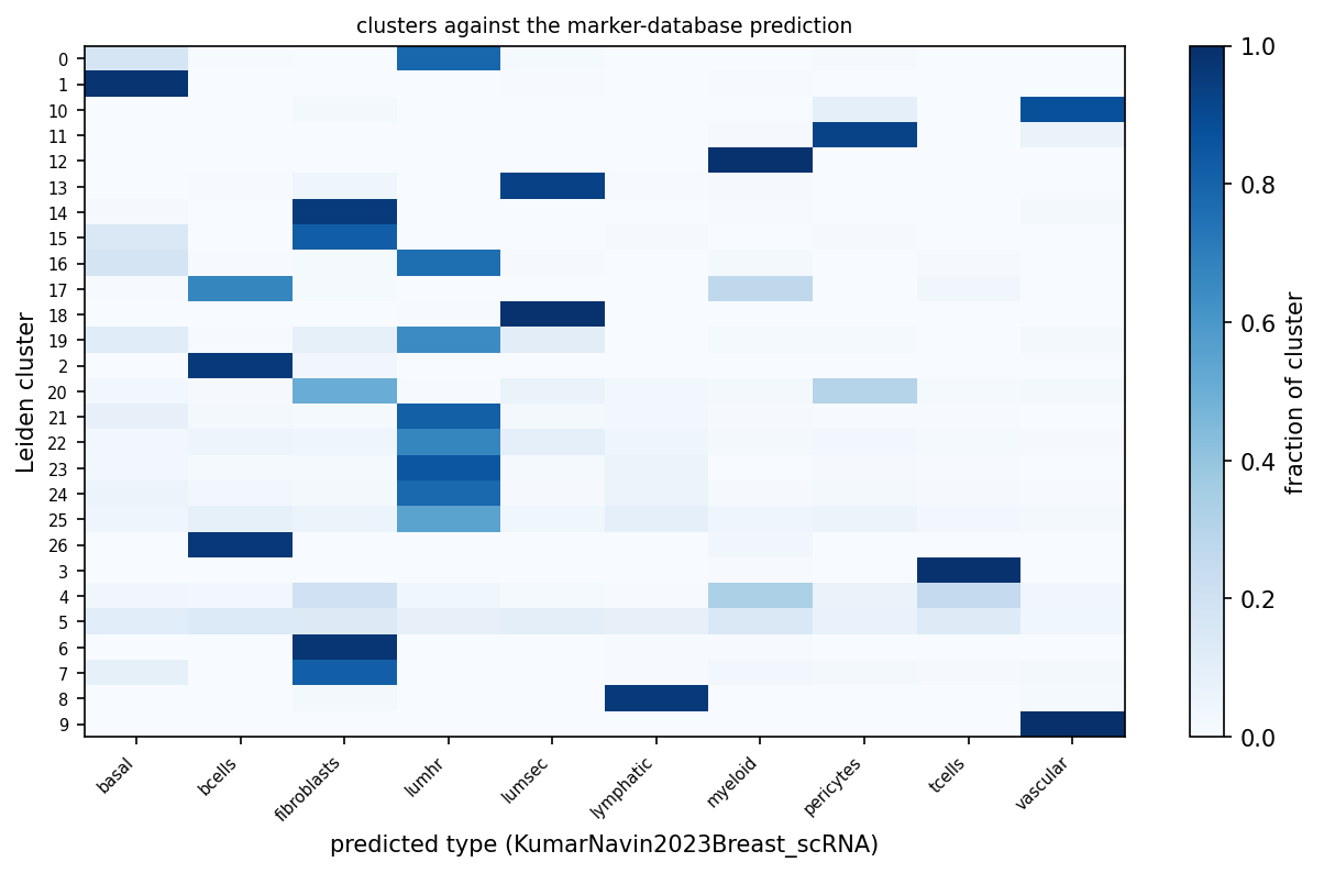
The two it gets wrong, and why that is the useful part

Two clusters are misassigned, and both failures are informative rather than random.

cluster’s markers	scRNA (10)	scRNA_fineAnno (58)	snRNA (11)
CPA3, CTSG, IL1RL1, MS4A2	lumsec (0.93)	Mast (1.00)	Mast (0.99)
PLIN4, GPD1, PLIN1, ADIPOQ	fibroblasts (0.51)	Fibro-matrix (0.32)	Adipocytes (0.97)

Mast cells (CPA3, MS4A2) are called lumsec at 0.93 by the 10-type reference — confidently, and wrongly. The reference has no mast category, so every mast cell is forced into the nearest label it does have. The 58-type annotation has Mast and calls them at 1.00.

Adipocytes (PLIN1, ADIPOQ) fail under both single-cell references and are recovered at 0.97 by the single-nucleus one. Adipocytes are large, lipid-filled and do not survive dissociation, so no scRNA atlas contains them. The assay of the reference decided the answer, not its granularity.

Two rules follow, and they apply to any marker-database prediction:

1. A prediction can only return a type the reference contains. There is no “none of these” class, so a missing type does not show up as low confidence — it shows up as a confident wrong answer. Check that your reference covers what is in your tissue before trusting the labels.
2. Match the reference’s assay and granularity to the question. sc versus sn decides whether adipocytes exist at all; 10 types versus 58 decides whether mast cells do.

One caveat specific to this section: Kumar/Navin is a normal breast atlas, so there is no malignant category. The tumour epithelium is assigned lumhr — the right lineage, and not a statement that those cells are normal.

4. What a 313-gene panel would have missed

To be explicit, because it is easy to misread: this dataset has 18,028 genes. The 313 below is not Atera — it is the comparison, the published Xenium human breast panel, used as the yardstick for what a conventional targeted run would have seen in the same tissue.

That panel was designed for exactly this tissue, so the comparison is a fair one: take the top 5 markers of each of the 27 clusters and ask how many are on it.

panel = set(piaso.pp.read_10x_h5("...breast_panel_matrix.h5").var_names)   # 313
names = pd.DataFrame(adata.uns["cosg"]["names"])

top5 = [g for g in names.iloc[:5].values.ravel() if isinstance(g, str)]
on = [g for g in top5 if g in panel]
len(on), len(top5), 100 * len(on) / len(top5)

(19, 135, 14.1)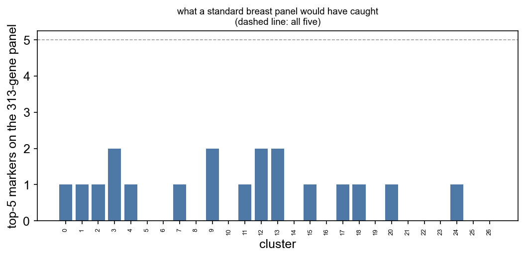

19 of 135 — 14.1%. And per cluster it is worse than the average suggests:

• No cluster has all five of its top markers on the panel. Not one.
• 12 of 27 clusters have none at all, meaning the panel offers nothing that would have distinguished them.

Some of what it misses:

CACNG4, COL17A1, JCHAIN, CXCL10, C7, COL10A1, MMRN1, PLVAP, HBB, LGI4, CSF1R

CSF1R is the canonical macrophage receptor. JCHAIN is the plasma-cell joining chain. CXCL10 names the mregDC state above and COL10A1 the matrix CAFs; COL17A1 names the basal/myoepithelial layer, the compartment whose loss defines invasion in breast tissue.

Read this carefully, because the obvious conclusion is slightly wrong. It does not mean the panel cannot find these cell types. A 313-gene panel designed for breast tissue contains other T-cell, macrophage and endothelial genes, and clustering on it would separate the major populations perfectly well. What it means is narrower and more useful:

The best marker for a population — the gene COSG ranks first when it may choose from the whole transcriptome — is usually not on the panel. And for the finer distinctions, arterial versus lymphatic endothelium, plasma-cell class, interferon state, the panel has no gene that separates them at all.

That is the trade. A panel is cheaper, has higher per-gene sensitivity, and answers the questions it was designed for. WTA answers the question you had not thought of yet — including “what is that cluster?”, which is the question you always end up asking.

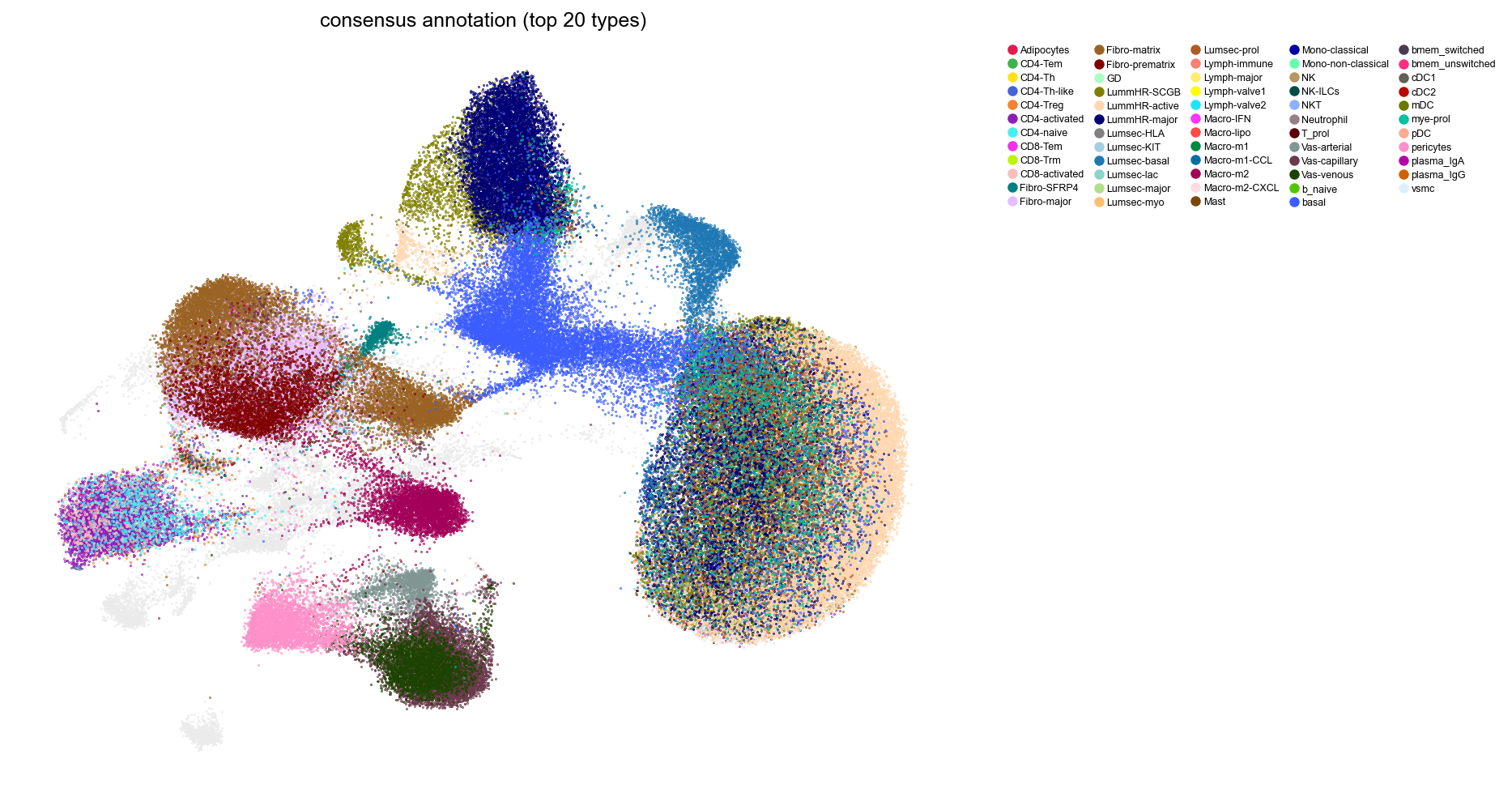
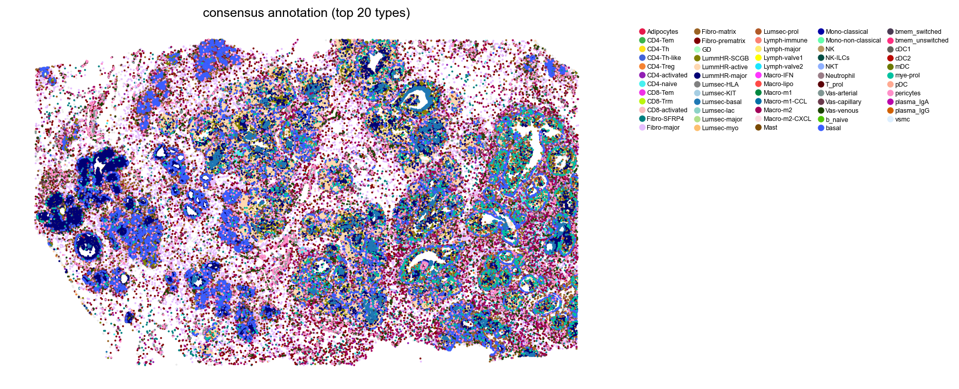
A consensus annotation, and why it is built per cluster

The fine reference fixes mast cells and the single-nucleus one fixes adipocytes, so the useful annotation combines them. The combination has to be made at the cluster level, not per cell:

fine = adata.obs["CellTypes_breast_fine"].astype(str)
sn   = adata.obs["CellTypes_breast_sn"].astype(str)
lei  = adata.obs["leiden"].astype(str)

# per-cell would be wrong -- see below
frac = (sn == "Adipocytes").groupby(lei).mean()
adipocyte_clusters = frac[frac >= 0.5].index

best = fine.copy()
best[lei.isin(adipocyte_clusters)] = "Adipocytes"
adata.obs["CellTypes_best"] = pd.Categorical(best)

Taking the single-nucleus call per cell would relabel 14,556 cells as adipocytes — and 13,017 of those sit inside the tumour clusters, which are not adipocytes by any reading. The snRNA reference has no malignant category and puts large, transcriptionally active cells somewhere; the somewhere happens to be adipocytes.

A cluster-majority rule rejects all of that and keeps the one population that really is adipose: cluster 20, 349 cells, at 97% agreement.

Transfer labels at the level the evidence supports. A per-cell argmax against an imperfect reference will always find somewhere to put a cell it has no category for; a cluster majority makes that failure visible instead of silent.

4b. The morphology image underneath

The bundle ships a DAPI morphology image, and putting the calls on top of it is the last check available: the cells should sit on nuclei, and the epithelial labels should follow duct walls.

import tifffile

with tifffile.TiffFile("morphology_focus/ch0000_dapi.ome.tif") as tf:
    levels = tf.series[0].levels
    level = next(i for i, l in enumerate(levels) if max(l.shape[-2:]) <= 8000)
    img = levels[level].asarray()
    if img.ndim == 3:
        img = img[0]                       # DAPI is channel 0
    full_w = levels[0].shape[-1]

scalef = (img.shape[-1] / full_w) / 0.2125     # micron -> stored pixel
p99 = np.percentile(img, 99)
img8 = np.clip(img.astype(np.float32) / p99 * 255, 0, 255).astype(np.uint8)

xy = np.asarray(adata.obsm["spatial"]) * scalef

Two details that will bite:

• morphology_focus is a four-channel OME series across four files. If you downloaded only ch0000, tifffile warns and zeroes the other three, and the array comes back (4, H, W) rather than (H, W) — take channel 0.
• The scale factor is the only number that must be exactly right: the coordinates are microns, full resolution is 0.2125 µm/px, and the pyramid level is a further downsampling. Here level 3 gives 3,506 × 5,817 px and scalef = 0.588.

Point size is the whole game in an overlay. At whole-section scale the points have to be almost invisible or they paint over the tissue you are checking against; zoomed in they can be large enough to read:

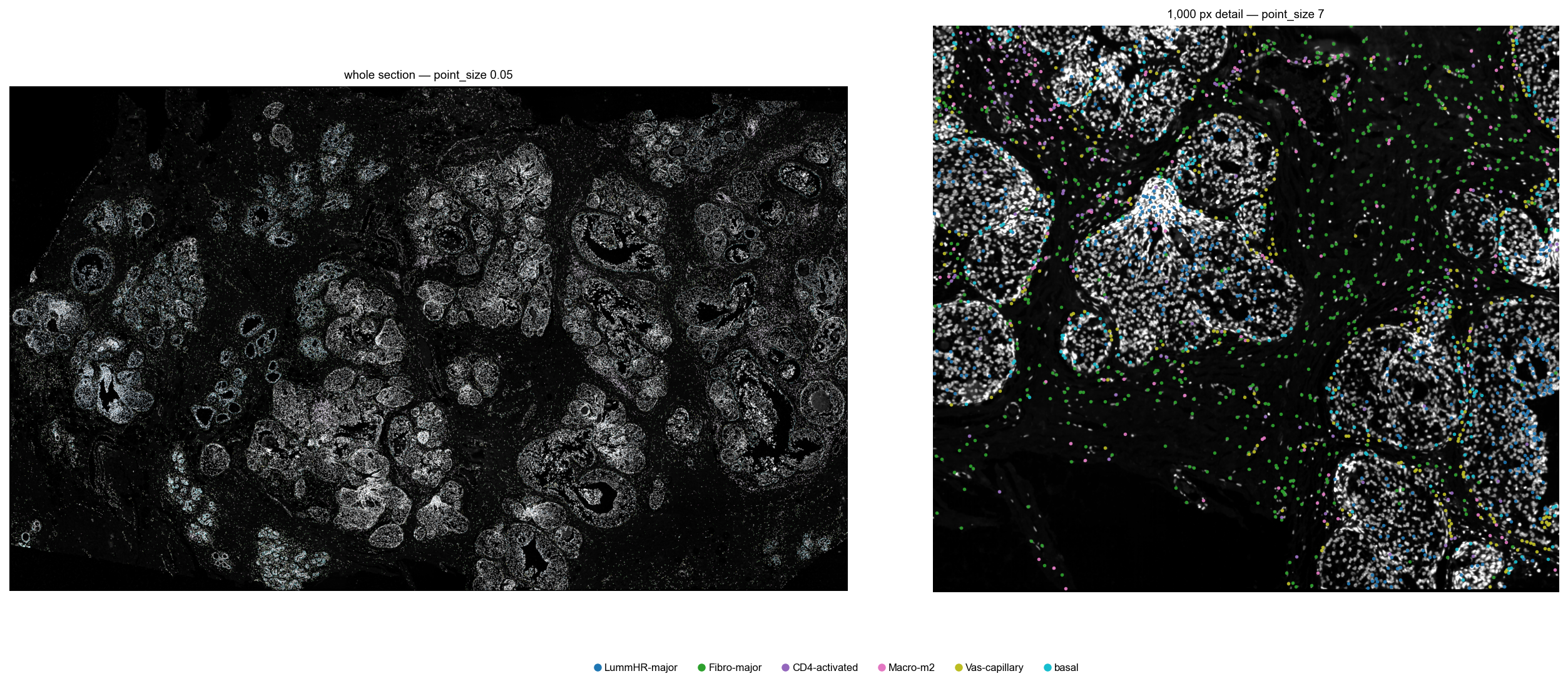
Left is the full section at s=0.05; right is a 1,000-pixel detail at s=7.

The detail is the registration check, and it passes on the cell type that makes it easiest to see: basal cells (cyan) trace the outside of the ducts, one cell thick, which is exactly where the myoepithelial layer sits — and Fibro-major (green) fills the stroma between ducts and stops at their edge. Neither of those was told where the ducts are; the DAPI image was never part of the analysis.

That single-cell-thick basal ring is also the feature whose loss defines invasion in breast pathology, so it is worth looking at directly rather than only counting it.

5. Canonical markers, in tissue space

adata.X = adata.layers["counts"].copy()
piaso.pp.normalize_log1p(adata)

genes = ["EPCAM", "ERBB2", "ESR1", "KRT8", "ACTA2", "PTPRC",
         "CD3E", "MS4A1", "CD68", "PECAM1", "COL1A1", "MKI67"]
piaso.pl.embedding(adata, color=genes, basis="spatial", point_size=0.45,
                   ncols=4, fix_coordinate_ratio=True)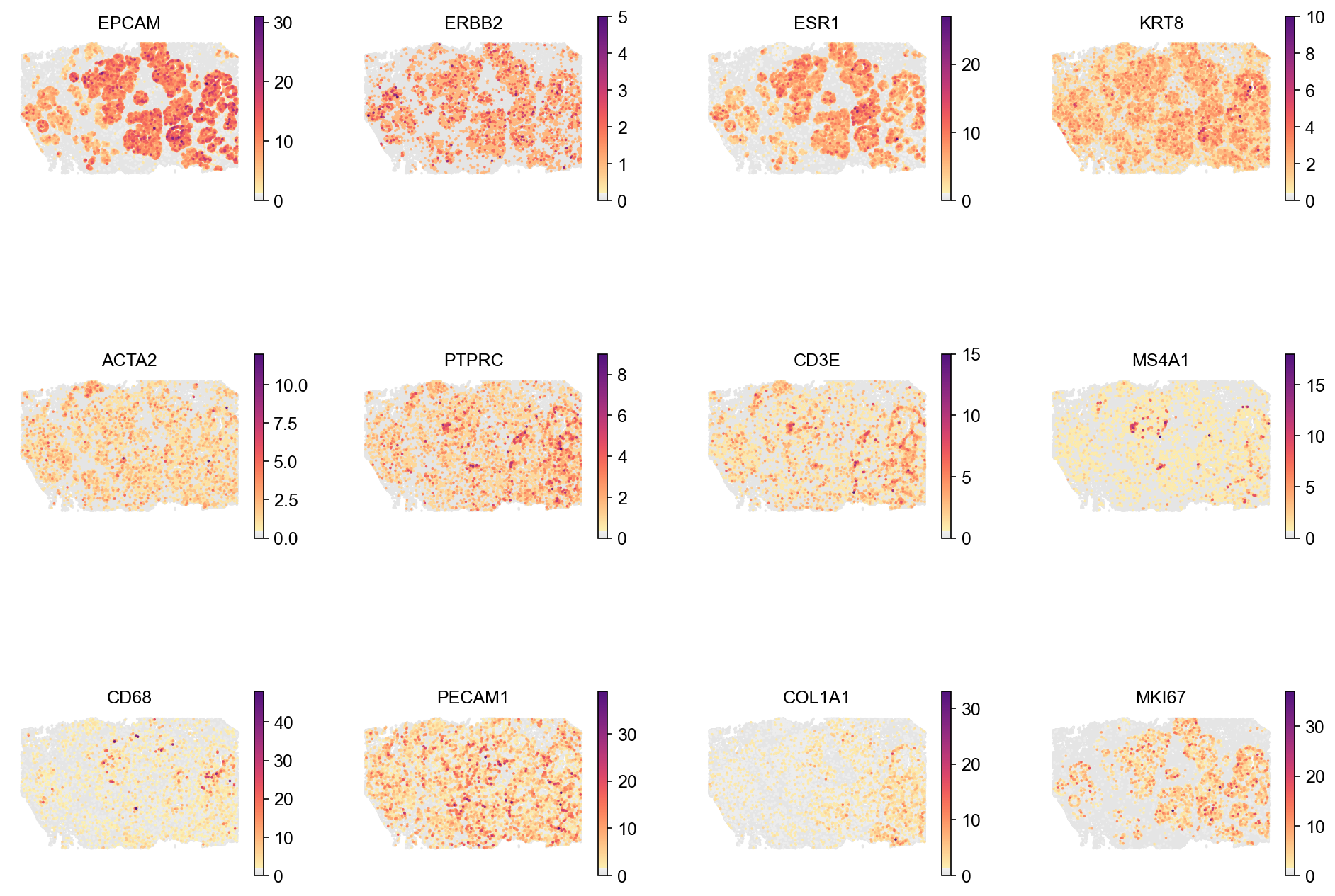

The tumour compartment (EPCAM, KRT8, ERBB2) forms solid nests; the stroma (COL1A1, ACTA2) surrounds them; the immune compartment (PTPRC, CD3E, MS4A1, CD68) is concentrated at the boundaries between the two, which is the spatial observation that dissociated data cannot make.

6. Which one should you run?

Both columns are measured from the two public datasets — the panel figures from Xenium human breast Rep 1, 167,780 cells.

	313-gene panel	Atera WTA
targets	313	18,028
median transcripts/cell	164	2,116
matrix size	~200 MB	~400 MB (h5), 55 GB bundle
gene choice	before the run	not required
best marker per cluster on-panel	by construction	—
finds what you did not plan for	no	yes

Use a panel when you know what you are measuring and want many sections cheaply. Use WTA when the point of the experiment is discovery — a tumour microenvironment, an unfamiliar tissue, or any question where “what is that cluster?” is a real question rather than a rhetorical one.

Everything downstream is identical either way: the code in this page and in the mouse brain tutorial differs only in the file paths.

Where to go next

• Xenium Prime 5K on mouse brain — the same pipeline explained step by step, checked against known anatomy.
• Xenium into a cytome — 170,000 cells × 18,028 genes is large enough that streaming starts to be worth it.
• Downstream on Xenium — KEGG pathways, LARIS ligand–receptor and cytorete regulons run on this very section, and the coverage measurement that says which of them a panel can support. The L–R answer is the one this page’s argument leads to: 2,831 usable pairs here against 11 on the 313-gene panel.
• PIASOmarkerDB — the marker database used above, and the other 35 studies in it.
• COSG markers — the marker step, and its p-values.
• LARIS — ligand–receptor analysis, which needs the receptor to be on the panel.