SCALAR: ligand-receptor interaction analysis

piaso.tl.runSCALAR asks, for every ordered pair of cell types and every known ligand–receptor pair: is the ligand specific to the sender and the receptor specific to the receiver, more than expected by chance?

The word doing the work is specific. SCALAR scores cell-type specificity, not mean expression, so a ligand every cell expresses cannot win. The null is built from genes matched to each query gene by expression and detected in the same cell type, so a highly expressed pair does not win either, and a gene present in a handful of the sender’s cells is not tested at all.

import numpy as np
import pandas as pd
import piaso, cosg

piaso.settings.set_figure_params(style="cell")

1. Data and an interaction database

SEA-AD middle temporal gyrus, 20,000 nuclei, 24 annotated subclasses:

adata = piaso.data.load_dataset("sea_ad_mtg_20k")
piaso.tl.infog(adata, layer="UMIs", n_top_genes=3000)

SCALAR needs an interaction database. piaso.data fetches CellChatDB on demand and caches it in ~/.piaso/data, the same way the genome and motif references work — nothing downloads until you ask:

lr = piaso.data.load_lr_database("human")     # or "mouse"
lr.shape, [c for c in lr.columns][:4]

((2951, 28), ['interaction_name', 'pathway_name', 'ligand', 'receptor'])

The mouse table is load_lr_database("mouse") — 3,105 pairs. Any table with a ligand column and a receptor column also works, so a curated in-house list can be passed straight to lr_pairs=.

What makes CellChatDB worth using rather than a bare pair list is the annotation column, which says by what mechanism each pair interacts:

lr["annotation"].value_counts()

Secreted Signaling       1200
Non-protein Signaling     746
ECM-Receptor              515
Cell-Cell Contact         490

Those are four different biological questions. A secreted ligand can act at a distance; an ECM-receptor pair means one cell is building matrix the other adheres to; cell-cell contact requires the two cells to touch. Pooling them answers none of the three cleanly, and §6 splits them.

2. The specificity matrix

SCALAR takes a genes × cell-types matrix of specificity scores. COSG produces exactly that, which means the same scores drive annotation and interaction analysis: one definition of “specific” across the analysis, not two.

cosg.cosg(adata, key_added="cosg", groupby="Subclass",
          n_genes_user=adata.n_vars, mu=10, remove_lowly_expressed=False)

names = pd.DataFrame(adata.uns["cosg"]["names"])
scores = pd.DataFrame(adata.uns["cosg"]["scores"])
spec = pd.DataFrame(0.0, index=adata.var_names, columns=names.columns)
for c in names.columns:
    spec.loc[names[c].values, c] = scores[c].values
spec.shape

(36601, 24)

Three choices in that call, each deliberate:

• n_genes_user=adata.n_vars asks COSG for every gene, not a top-N — the matrix needs a score for any gene that might appear in the database. A top-N result pivoted into a matrix leaves NaN for every gene outside each type’s list, and runSCALAR refuses NaN rather than score it.
• mu=10. COSG’s regularisation weights a gene’s off-target signal by mu. The test is nearly indifferent to it — within-pair rankings agree at Spearman > 0.99 between mu=1 and mu=100 — but the score column is not: at mu=100 five in six ligand–receptor genes fall below a tenth of their mu=1 value, because a ligand shared by two related subclasses (SST across Sst and Sst Chodl, GAD2 across every interneuron) counts as off-target, and the plots below would be sized by numbers with four leading zeros. mu=10 keeps that penalty at a few-fold and every score readable.
• remove_lowly_expressed=False. COSG’s own detection filter marks genes it drops with −1, and two such sentinels multiply to +1 — the largest product a table can hold. SCALAR applies the same 10 % detection floor itself, in the test rather than in the matrix (§3), and raises on negative input so the sentinels cannot reach it. A matrix built with the filter on and the sentinels set to 0 gives the same result; there is just no reason to build one.

The scores go in raw. Dividing each cell type’s column by a constant — an IQR, a maximum — changes nothing, because the observed product and every product in its null scale together; cosg.iqrLogNormalize adds a log1p on top, which compresses the top of each column and costs a quarter to a third of the calls. Scores compare within a sender–receiver pair, and within a pair a per-column scale is invisible.

3. Run it

res = piaso.tl.runSCALAR(adata, specificity_matrix=spec, lr_pairs=lr,
                         ligand_col="ligand", receptor_col="receptor",
                         annotation_col="Subclass", layer="infog",
                         groupby="Subclass")
res.shape, list(res.columns)

((1691712, 17),
 ['ligand', 'receptor', 'sender', 'receiver',
  'ligand_specificity', 'receptor_specificity',
  'interaction_score', 'specificity_geomean',
  'p_value', 'testable', 'null_matchability', 'null_mean', 'log2_enrichment',
  'ligand_expressed_pct', 'receptor_expressed_pct',
  'p_value_fdr', 'nlog10_p_value_fdr', 'call_breadth'])

1.69 million candidate interactions — ~2,900 usable LR pairs × 576 ordered cell-type pairs — of which 290,751 (17 %) are tested. The rest fail the detection floor: an interaction is tested only if the ligand is detected in at least 10 % of the sender’s cells and the receptor in at least 10 % of the receiver’s (expressed_pct=0.1, counted on layer; INFOG and log1p leave the zeros where the counts put them, so the fraction is the same from any of them). groupby names the cell-type column so the floor can be counted per type. Rows that fail come back with testable = False, p_value = 1, and stay out of FDR; ligand_expressed_pct and receptor_expressed_pct carry the fractions the floor was applied to, so every call can be checked against it.

The floor is applied in the test, not by zeroing the matrix. Each gene’s matched controls are drawn from genes that are also detected at 10 % in the same cell type, so the null never contains a control that is not expressed where it is used. Zeroing lowly-detected genes in the matrix instead would leave the observed pair conditioned on passing the floor while its controls are zeroed wherever they fall below it; most of the null becomes zeros and the p-value drifts toward “detected in more cells than its peers”. Measured on this dataset, a quarter of the calls that approach makes are significant only because of the zero padding.

The p-values are exact, not sampled: each interaction’s null is the fully enumerated 100 × 100 support of matched-ligand × matched-receptor score products, so the result is deterministic — no n_permutations, no seed sensitivity, and a hard floor of 1/10,001. FDR is applied per sender–receiver pair independently, which matters: correcting globally across 576 pairs would bury every result in a single enormous multiple-testing penalty for questions that were never one family.

Three columns give the score a magnitude. interaction_score is the statistic the test uses — the product of the ligand’s specificity in the sender and the receptor’s in the receiver, both returned alongside it — and a product of two numbers below 1 is smaller than either, so a pair of two 0.02 specificities scores 0.0004. specificity_geomean is their geometric mean: a monotone function of the product, so it ranks exactly as the score does, but it lives on the specificity scale (that pair reads 0.02), and the plots below are sized by it. log2_enrichment is the observation over null_mean, the mean of the interaction’s own 100 × 100 matched null: how far the pair sits above what expressed, expression-matched gene pairs achieve between these two cell types. It is the one number that compares across sender–receiver pairs, because every pair is referenced to its own null; raw scores are not, because specificity is calibrated within a cell type.

Two more diagnostic columns come with every run. null_matchability measures whether the matched-gene null was fair to this interaction: 0.5 is ideal; ≥ 0.99 means the gene sits above its entire matched set in mean expression, so it beats its null arithmetically and the p-value overstates. A warning names such genes when they are called; on this run, with controls drawn among expressed genes, none is. call_breadth is the fraction of the sender–receiver grid an interaction is called in: genuinely cell-type-specific results are narrow (median 1.6 % of the grid among the calls here), and a pair called across most of the grid is a ubiquity signature whatever its p-value.

It reports what it dropped:

Filtered out 14 LR pairs that were not found in both the AnnData object
and the specificity matrix.
  - Detection floor 10% on layer 'infog': 7,511-16,660 genes per cell type
    form the matched universes
  - 290,751 of 1,691,712 interactions clear the detection floor in both
    cell types and were tested

Changed since PIASO 1.1.0

The archived v1.1.0 version of this tutorial reported 14,052 significant interactions on the same data; this page reports 1,464. Three things changed, each for a stated reason. The null is enumerated exactly over 100 × 100 matched products instead of sampled 1,000 times over 30 × 30 — the sampled null at k = 30 saturated small groups, and this change alone removes more than half the calls. The specificity matrix goes in raw at mu=10 instead of IQR-then-log-normalised at mu=100 — the log step removed calls without changing any ranking. And the detection floor above now exists — a third of the remaining calls rested on a ligand or receptor detected in under 10 % of its cell type. Every number on this page comes from the current method.

4. What comes out

Top significant interactions, and each one is checkable:

ligand	receptor	sender	receiver	score	geomean	log2 enrichment	FDR
PTPRC	CD22	Microglia-PVM	Oligodendrocyte	0.747	0.864	3.4	0.034
COL1A2	SDC4	VLMC	Astrocyte	0.554	0.745	9.0	0.010
COL1A2	ITGA2	VLMC	Oligodendrocyte	0.531	0.729	7.7	0.032
COL1A2	CD44	VLMC	Astrocyte	0.314	0.560	8.3	0.010
COL6A3	SDC4	VLMC	Astrocyte	0.239	0.488	6.6	0.044
VIP	SCTR	Vip	Vip	0.149	0.386	9.7	0.019
LAMB1	ITGA2	L2/3 IT	Oligodendrocyte	0.120	0.346	5.9	0.020
LAMB1	ITGB4	L2/3 IT	Astrocyte	0.087	0.295	6.6	0.019
NPY	GPR83	Sst Chodl	L2/3 IT	0.075	0.274	14.2	0.008
LAMB1	CD44	L2/3 IT	Astrocyte	0.071	0.266	6.6	0.019

Read down that column of senders. VLMC — vascular leptomeningeal cells — dominate the collagen signalling, which is what they do: they build the extracellular matrix of the meninges and perivascular space, and collagens I and VI land on syndecan-4, CD44 and integrin α2. PTPRC → CD22 heads the table: CD45 on microglia against CD22, which in this tissue is detected in 78 % of oligodendrocyte nuclei and almost nowhere else, so both ends of the pair are sharp. VIP → SCTR is the one autocrine entry, VIP interneurons onto a receptor they themselves express. And NPY → GPR83 is the first neuronal peptide in the list, from the small Sst Chodl subclass that §5b returns to.

None of that was supplied. The inputs were a count matrix, a subclass label and a public interaction table.

Now read the enrichment column against the score column. PTPRC → CD22 has the largest score in the table and the smallest enrichment: its controls — expressed, expression-matched genes in microglia and oligodendrocytes — are themselves fairly specific, so 0.75 is only ten times its null (2³·⁴). NPY → GPR83 scores a tenth of that and sits 19,000 times above its null. Sorted by enrichment instead, the top of the table is Sst Chodl’s peptides and monoamine machinery from the first row to the tenth. Among all 1,464 calls the enrichment runs from 4.5 (10th percentile) to 9.1 (90th), median 6.6; among everything tested, the median is −3.

The whole result fits in one picture — how many significant pairs each sender has with each receiver:

import matplotlib.pyplot as plt

counts = (sig.groupby(["sender", "receiver"]).size()
             .unstack(fill_value=0)
             .reindex(index=sorted(spec.columns),
                      columns=sorted(spec.columns), fill_value=0))

fig, ax = plt.subplots(figsize=(9, 7.5))
im = ax.imshow(counts.values, cmap="Purples", aspect="auto")
ax.set_xticks(range(counts.shape[1]))
ax.set_xticklabels(counts.columns, rotation=90, fontsize=7)
ax.set_yticks(range(counts.shape[0]))
ax.set_yticklabels(counts.index, fontsize=7)
ax.set_xlabel("receiver"); ax.set_ylabel("sender")
fig.colorbar(im, ax=ax, label="significant LR pairs", shrink=.8)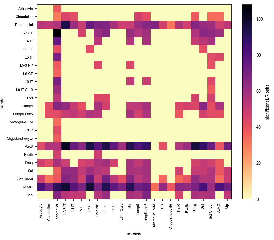

Rows are senders and columns receivers, so the matrix is deliberately asymmetric: A→B and B→A are different questions and SCALAR answers both.

5. Read it at the level of the question

Individual pairs are noisy; the aggregate is what most analyses want:

sig = res[res["p_value_fdr"] < 0.05]
sig.groupby(["sender", "receiver"]).size().sort_values(ascending=False).head(6)

sender       receiver
VLMC         L6 IT Car3      25
VLMC         Astrocyte       22
VLMC         Sst             21
Sst Chodl    L6b             17
L6b          Lamp5 Lhx6      17
Sst Chodl    L5 IT           17

A caution worth stating plainly: interaction counts track cell-type abundance and specificity sharpness, not just biology. VLMC heads the list three times over because its collagen markers are unusually sharp, not because it necessarily signals more, and Sst Chodl is a small subclass whose peptides are exclusive to it. Compare pairs of comparable size, or normalise, before concluding that one cell type “talks more”.

5b. Interneurons onto excitatory neurons

The pairs above are dominated by vasculature and glia, because those cell types have the sharpest markers. Neurons are the more interesting question, and they have to be asked directly:

EXC = ["L2/3 IT", "L4 IT", "L5 IT", "L6 IT", "L5 ET", "L6 CT",
       "L5/6 NP", "L6b", "L6 IT Car3"]
INH = ["Sst", "Pvalb", "Vip", "Lamp5", "Lamp5 Lhx6", "Sncg",
       "Chandelier", "Pax6", "Sst Chodl"]

onto_exc = sig[sig["sender"].isin(INH) & sig["receiver"].isin(EXC)]
onto_exc["sender"].value_counts()

Sst Chodl     121
Pax6           54
Lamp5 Lhx6     38
Sncg           25
Vip            20
Lamp5          13
Pvalb          10
Chandelier      4
Sst             2

287 significant interneuron → excitatory interactions, and they are not spread evenly. Before reading biology into that ordering, note the caution from §5: Sst Chodl is a small subclass with very sharp markers, and count tracks marker sharpness as much as it tracks signalling.

Peptides from one class, GABA machinery from the other

Put two interneuron classes onto the same receiver, so the receptor side is held constant and only the sender changes:

pairs = ["Sst Chodl@L6b", "Pvalb@L6b"]
sub = sig[sig["CellTypeXCellType"].isin(pairs)]
sub.groupby("CellTypeXCellType")["ligand"].agg(lambda s: sorted(set(s)))

Pvalb@L6b        [FGF9, GAD1, GAD2, SLC6A6]
Sst Chodl@L6b    [CORT, DDC, GHRH, NPY, NTN4, SST, WNT7A]

Sst Chodl signals with peptides. Its own neuropeptides carry the list — NPY → NPY1R and NPY5R, SST → SSTR2 and SSTR3, CORT → SSTR2, GHRH → VIPR1 — with DDC, the enzyme that makes dopamine and serotonin, onto a spread of monoamine receptors, and a WNT7A triplet. Seventeen calls, nine of them secreted signalling.

Pvalb has almost nothing that is its own. Four calls, and three of them are GABA machinery — GAD1, GAD2 and the transporter SLC6A6 onto the GABA-A subunit GABRA5 — plus FGF9 → FGFR1. That is a negative result and it is the biologically sensible one: parvalbumin is a calcium buffer, not a ligand, and PV cells are defined by fast GABAergic transmission through machinery every inhibitory neuron shares. A method that invented a distinctive PV ligand repertoire here would be wrong.

y_max = sub["specificity_geomean"].max() * 1.15

piaso.pl.plotLigandReceptorInteraction(
    interactions_df=sig, specificity_df=spec, cell_type_pairs=pairs,
    col_interaction_score="specificity_geomean",
    ligand_receptor_sep="-->", top_n=15, y_max=y_max,
    heatmap_cmap="Purples", shared_legend=True,
    fig_width=20, fig_height_per_pair=6)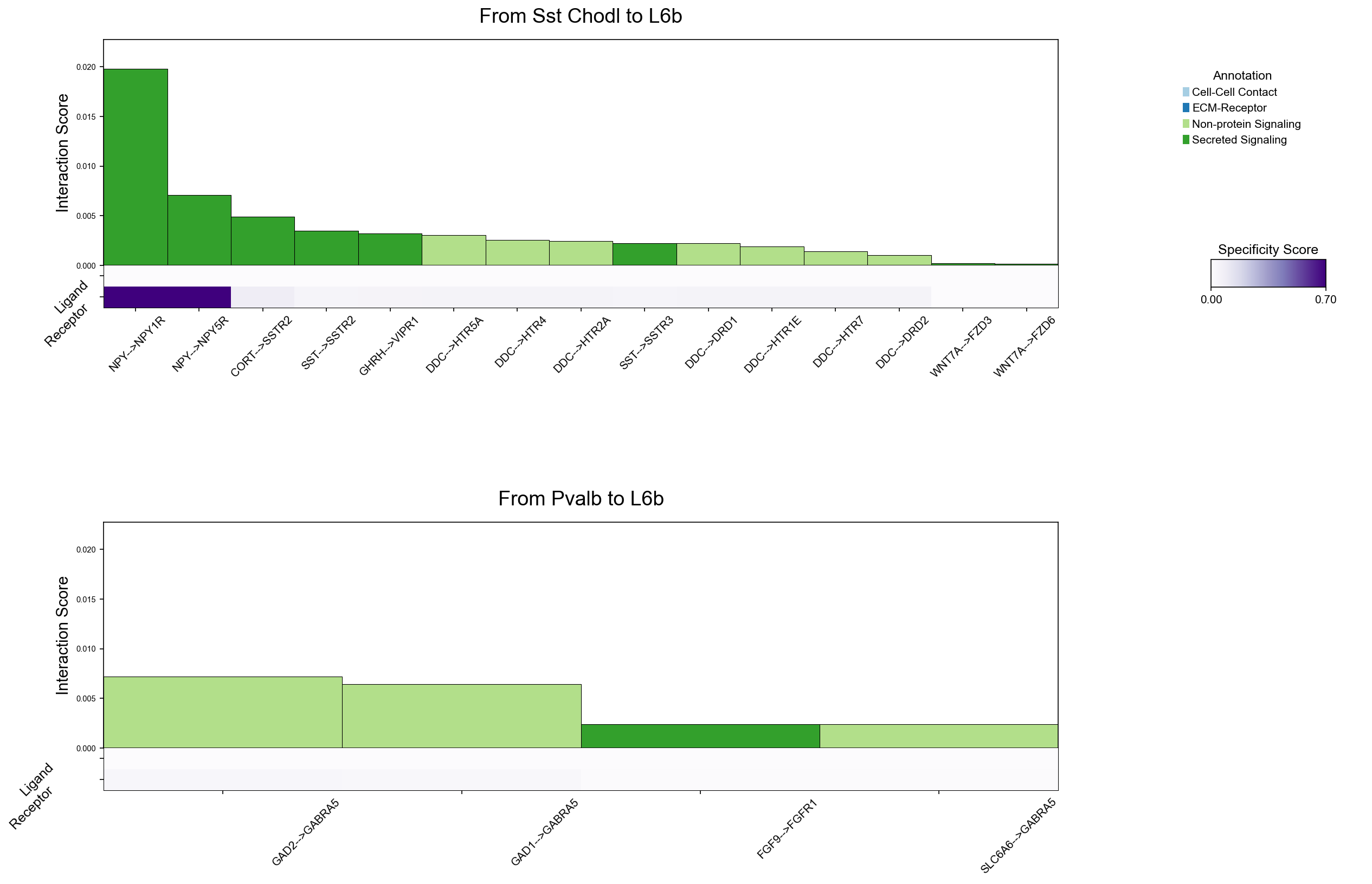

The bars are the geometric-mean specificity, and y_max is set from the data: even on that scale the neuronal pairs sit at 0.02 against the collagen panels’ 0.75, and reusing one axis would flatten all of this to nothing.

And the Sst subclass itself, the canonical somatostatin interneuron? Two calls onto excitatory neurons, both shared with Pvalb. Its SST → SSTR2 onto L5 IT has p = 0.0005 — the second-best p-value among the 540 interactions tested for that pair — but an FDR of 0.13, and the reason is visible in the ligand_expressed_pct column: the SST transcript is detected in 27 % of Sst nuclei against 84 % of Sst Chodl nuclei in this snRNA-seq data, so its specificity score is small and its rank in the pair not high enough to clear 0.05. From Sst Chodl the same pair is called at FDR 0.007. The floor is doing what it should — it does not veto SST from Sst (27 % clears 10 %) — and the p-value is honest about how much of the transcript the nuclei actually caught.

Interaction scores compare within a sender–receiver pair, not across

The score is a product of two specificity scores, and specificity is only calibrated within a cell type — a small, sharply-marked population reaches high scores because its markers are exclusive, not because it signals more. So “COL1A2→SDC4 from VLMC to astrocytes has a geometric-mean specificity of 0.74 and NPY→NPY1R from Sst Chodl to L6b has 0.02” is not a statement that the first interaction is thirty-seven times stronger — and by enrichment over their own nulls it is the other way round, 2⁹ against 2¹²·⁷.

Read scores down a column: which ligand–receptor pairs matter between these two cell types. That ordering is stable — it survives any monotone rescaling of the specificity matrix. To compare across pairs, use log2_enrichment, which references every interaction to its own matched null, or the counts of significant interactions (§4) — never the score magnitudes — and remember the caution in §5 that counts track marker sharpness too.

Half of this is “Non-protein Signaling”, and it means something different

Look at the annotation colours: many of the neuronal bars are Non-protein Signaling, not Secreted Signaling. GAD1, GAD2 and SLC6A6 are a synthesis enzyme and transporters; DDC is a synthesis enzyme. None of them is a secreted ligand.

CellChatDB carries them as stand-ins for transmitters that have no gene of their own — there is no “GABA” or “serotonin” gene to put on the ligand side — so GAD2 → GABRA5 means “this cell makes GABA and that one can receive it”, not that GAD2 binds GABRA5. It is a reasonable convention and it is why the neuronal results are legible at all, but it is a different kind of claim from SST → SSTR2, where the ligand really is the protein named.

The annotation column tells you which you are looking at, and it is worth filtering on when the distinction matters.

6. Plot one pair properly

A ranked table does not show why an interaction scored. plotLigandReceptorInteraction does: a bar for the interaction score, and directly beneath it the two specificity scores that produced it — the ligand’s in the sender, the receptor’s in the receiver. An interaction with a tall bar and a pale square underneath is one gene carrying the pair.

It wants three derived columns, all of them one line (the two specificities it reads, ligand_specificity and receptor_specificity, are already in the table):

sig = res[res["p_value_fdr"] < 0.05].copy()

sig["CellTypeXCellType"] = sig["sender"] + "@" + sig["receiver"]
sig["ligandXreceptor"] = sig["ligand"] + "-->" + sig["receptor"]

ann = (lr.drop_duplicates(subset=["ligand", "receptor"])
         .set_index(["ligand", "receptor"])[["annotation", "pathway_name"]])
sig = sig.join(ann, on=["ligand", "receptor"])

pairs = ["Sst Chodl@L5 IT", "Pax6@Sst"]
y_max = sig[sig["CellTypeXCellType"].isin(pairs)]["specificity_geomean"].max() * 1.15

piaso.pl.plotLigandReceptorInteraction(
    interactions_df=sig, specificity_df=spec, cell_type_pairs=pairs,
    col_interaction_score="specificity_geomean",
    ligand_receptor_sep="-->", top_n=30, y_max=y_max,
    heatmap_cmap="Purples", shared_legend=True,
    fig_width=20, fig_height_per_pair=6)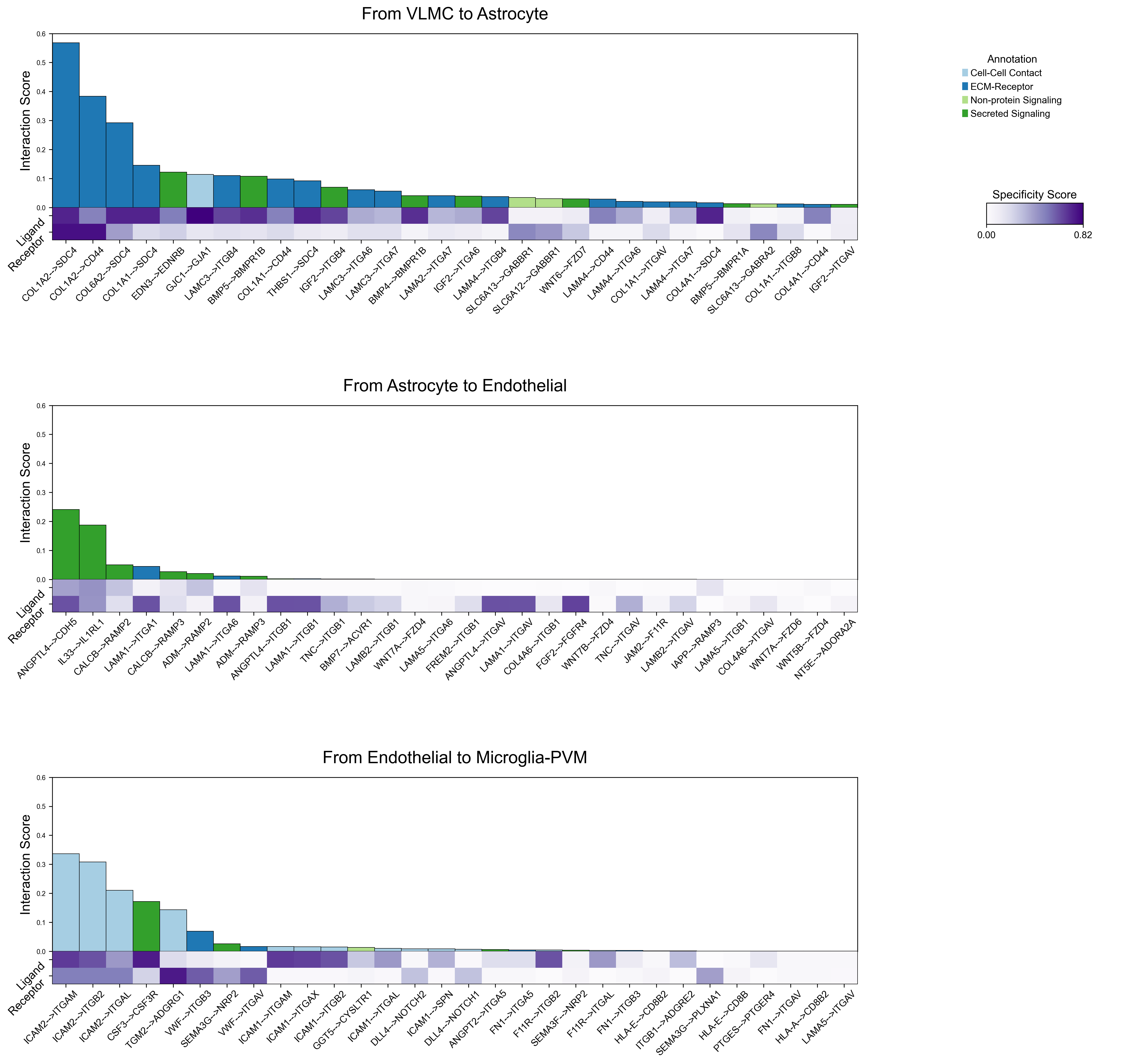

Two neuronal pairs, bars sized by the geometric-mean specificity, and the colour of each bar says by what mechanism:

• Sst Chodl → L5 IT is green and grey: secreted peptides and non-protein transmitters. NPY onto three of its receptors (NPY1R, NPY2R, NPY5R), CORT and SST onto SSTR2, GHRH → VIPR1, and DDC onto dopamine and serotonin receptors. Look at the heatmap underneath the NPY bars: the ligand square is dark (specificity 0.70) and the receptor squares are pale (0.001–0.007). NPY is carrying those pairs almost alone — which is true, and is exactly the case the plot exists to show.
• Pax6 → Sst is mixed: RELN → LRP8 is ECM-receptor (reelin onto ApoER2), NTF3 → NTRK2 secreted, and SLC17A8 and SLC1A1 onto kainate receptors are the glutamate stand-ins from the caution above.

Set y_max from the data. It defaults to 10, and these geometric means top out at 0.07, so leaving the default draws every bar as a sliver against an empty axis.

7. Split by mechanism

annotation is a filter, and filtering before plotting turns a mixed panel into a controlled comparison. Same sender, two receivers, one mechanism:

ecm = sig[sig["annotation"] == "ECM-Receptor"]
len(ecm)

458

pairs = ["VLMC@Astrocyte", "VLMC@L2/3 IT"]
y_max = ecm[ecm["CellTypeXCellType"].isin(pairs)]["specificity_geomean"].max() * 1.15

piaso.pl.plotLigandReceptorInteraction(
    interactions_df=ecm, specificity_df=spec, cell_type_pairs=pairs,
    col_interaction_score="specificity_geomean",
    ligand_receptor_sep="-->", top_n=30, y_max=y_max,
    heatmap_cmap="Purples", shared_legend=True,
    fig_width=20, fig_height_per_pair=6)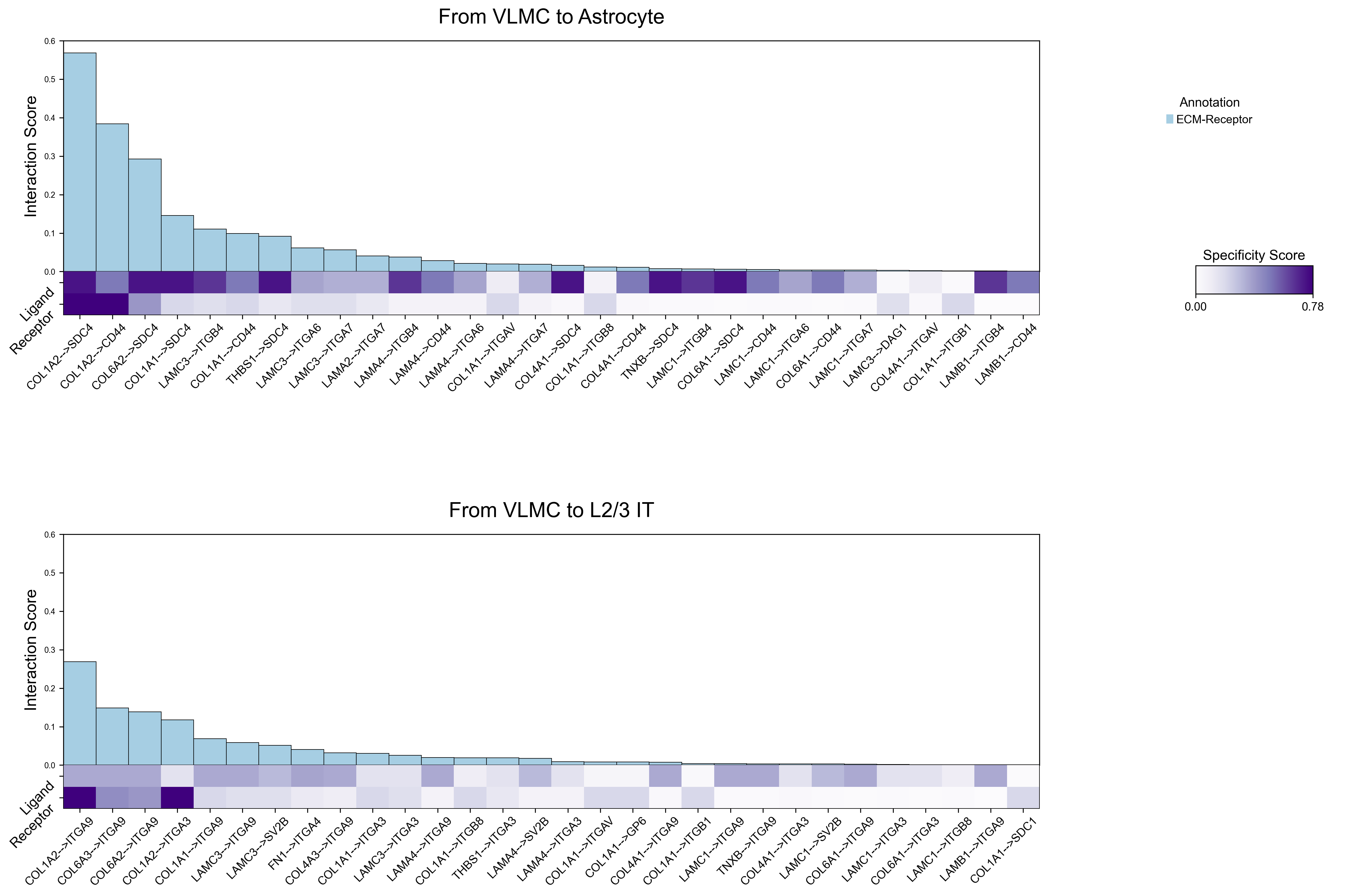

The ligands barely change — VLMC sends COL1A2, COL6A3, COL6A2 and COL1A1 to both. The receptor changes completely. Astrocytes receive them on SDC4, CD44 and ITGA7; L2/3 IT neurons receive the same collagens on ITGA9 (eleven of the fourteen calls) and ITGA3. One matrix source, two adhesion systems, and the split only appears because the mechanism class was held constant.

That is the argument for keeping annotation rather than reducing the database to a bare pair list.

8. One pair in full detail

plotLigandReceptorLollipop puts the ligand’s specificity above the axis and the receptor’s below, so the two halves of each interaction are read at once, and adds a third variable as circle size.

Circle size comes from col_circle_size, default avg_log2FC: any per-row effect size you care about. Here it is the ligand’s fold change between high-pathology and not-AD donors, which turns a description of the cortex into a question about the disease:

adc = adata.obs["Overall AD neuropathological Change"].astype(str)
hi, lo = adc.isin(["High", "Intermediate"]), adc.isin(["Not AD", "Low"])
# CP10K means per sender cell type, high-pathology vs not-AD
sig["avg_log2FC"] = ...     # see the note below

piaso.pl.plotLigandReceptorLollipop(
    sig, cell_type_pairs=["Sst Chodl@L5 IT"], top_n=30,
    col_interaction_score="specificity_geomean",
    col_cell_type_pair="CellTypeXCellType", sort_by_category=True,
    fig_height_per_pair=4.5, fig_width=16, vertical_layout=False,
    background_colors=True, logfc_range=1, base_circle_size=30,
    color_labels_by_annotation=True)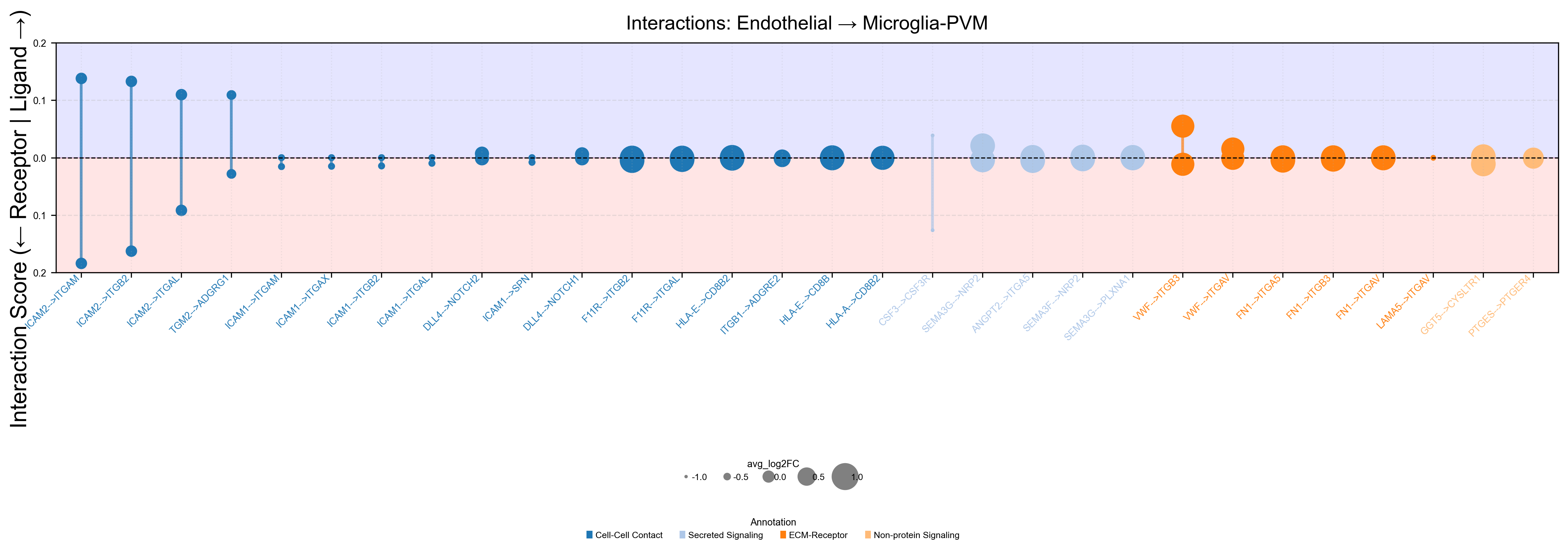

sort_by_category=True groups by mechanism, so the panel reads left to right as secreted → non-protein, and the stems are the geometric-mean specificity. The NPY stems are the tall ones above the axis and nearly flat below it: one side of each pair is carrying the score alone, which is exactly the case where a nominally significant interaction is worth less than its p-value suggests — and it is why SST → SSTR2, a short stem with both halves present, has the highest enrichment in the panel (2¹²·⁶) while NPY → NPY1R, the tallest, has 2¹¹·⁹. The circles add the disease axis: in Sst Chodl nuclei from high-pathology donors, GHRH is up 1.1 log2 units, CORT 0.75, DDC 0.53 and NPY 0.34, while SST itself is flat (0.03).

Without a col_circle_size column the function warns and draws every circle at one size; the plot is still correct, it just has one variable fewer.

The fold change used above:

X = adata.layers["UMIs"].tocsr()
cp10k = X.multiply(1e4 / np.asarray(X.sum(1)).ravel()[:, None]).tocsr()
gidx = {g: i for i, g in enumerate(adata.var_names)}

lfc = {}
for ct in spec.columns:
    m = (adata.obs["Subclass"] == ct).values
    a = np.asarray(cp10k[m & hi.values].mean(0)).ravel()
    b = np.asarray(cp10k[m & lo.values].mean(0)).ravel()
    lfc[ct] = np.log2((a + 0.1) / (b + 0.1))

sig["avg_log2FC"] = [lfc[r.sender][gidx[r.ligand]] for r in sig.itertuples()]

14,600 nuclei from high or intermediate pathology against 5,400 from not-AD or low. The strongest AD-up ligand among significant interactions is endothelial SEMA3G (log2FC 3.7), signalling onto plexins on Sst Chodl, Lamp5 Lhx6 and endothelium itself, but note its interaction scores are tiny (10⁻⁵ to 10⁻⁴). A large fold change and a small specificity score are different statements, and the lollipop is showing you both at once rather than letting one stand in for the other.

9. Narrow the question

Scoring all 576 pairs is cheap, but if you have a hypothesis, say so — the p-values are then spent on the comparison you care about:

res = piaso.tl.runSCALAR(adata, specificity_matrix=spec, lr_pairs=lr,
                         ligand_col="ligand", receptor_col="receptor",
                         annotation_col="Subclass",
                         sender_cell_types=["Astrocyte", "VLMC", "Endothelial"],
                         receiver_cell_types=["Microglia-PVM"],
                         layer="infog", groupby="Subclass")

8,811 candidate interactions, 900 of them clearing the floor, in nine seconds.

Parameters worth knowing

parameter	what it changes
expressed_pct	the detection floor (default 0.1): a gene must be non-zero in at least this fraction of a cell type’s cells to be tested there, and matched controls are drawn from genes that clear the same floor in the same type. None turns it off and reproduces the unfloored test exactly.
groupby	the cell-type column the floor is counted on; its labels must be the columns of the specificity matrix. Required when the floor is on.
statistic	"product" (default): one very specific gene can carry a pair. "min": the smaller of the two specificities, so both sides must beat the controls’ weaker sides — the “are both specific” question, with an exact null that factorises into two one-sided counts.
enrichment_pseudocount	added to observation and null mean in log2_enrichment so a near-zero null cannot give an infinite value (default 10⁻⁶).
n_nearest_neighbors	how many matched control genes per side (default 100). The null is the fully enumerated k × k product support, so this is the only knob for the p-value floor, 1/(k²+1) — 1/10,001 at the default.
n_permutations	deprecated — ignored with a warning. The null is enumerated exactly; sampling it only added noise, and raising this never lowered the floor.
sender_cell_types / receiver_cell_types	restrict the comparison.
prefilter_fdr	exclude score-0 pairs (degenerate nulls) from FDR. On by default at threshold 0; any threshold above 0 selects on the test statistic itself and warns.
layer	which matrix supplies expression — the space control genes are matched in, and the matrix the detection floor is counted on. infog here.
random_seed	kept for API stability; the p-value path no longer uses randomness.

Related

• Gene set scoring (PIASOscore): the same control-set idea, applied to gene sets rather than gene pairs.
• LARIS is the spatial counterpart: when cells have coordinates, physical proximity constrains which interactions are possible, and LARIS uses it. Same databases, per-cell answer.
• Datasets and genome references: the rest of what piaso.data fetches on demand.