cytorete on an AnnData: the same regulons, in memory

The regulons tutorial runs on a .cytome, because that is what an atlas usually is. Everything on that page works on an AnnData too — this one runs the identical chain on the h5ad of the same dataset and reports where each result lands, which is the only thing that actually differs between the two containers.

If you already know the cytome page, the short version is: swap the object, change nothing else, and read adata.obsm / adata.uns instead of ds.embeddings / ds.metadata.

pip install cytorete        # pulls piaso-tools>=1.2.2, cosg, cytome

1. Inputs

The same three files, and the h5ad instead of the cytome:

import piaso, cytorete

jaspar = piaso.data.fetch_jaspar()            # JASPAR CORE vertebrates MEME
twobit = piaso.data.fetch_2bit("hg38")        # genome sequence, ~800 MB, once
piaso.data.fetch_genome("hg38")               # TSS BED among the references

adata = piaso.data.load_dataset("sea_ad_mtg_20k")     # 20,000 × 36,601
piaso.settings.set_figure_params(style="cell")

The 2bit is the real cost of this tutorial and it is worth saying before you start: ~800 MB, downloaded once, cached in ~/.piaso/data. Nothing else here is large.

An embedding to draw on, and the normalisation the regulon step will score against:

piaso.tl.infog(adata, layer="UMIs", n_top_genes=3000)
piaso.tl.runSVD(adata, layer="infog", n_components=50, key_added="X_svd")
piaso.tl.neighbors(adata, use_rep="X_svd", n_neighbors=15)
piaso.tl.umap(adata, use_rep="X_svd")

piaso.tl.umap writes adata.obsm["X_umap"] and returns nothing, as of 1.2.4 — on both backends. If you are used to binding its return value, that is the one thing on this page that changed.

2. One call, same as the cytome

cytorete.tl.inferRegulon(adata, "hg38", "Subclass",
                         jaspar_path=jaspar, twobit_path=twobit)

No tf_list: every TF in the motif database that is expressed here, which is the only set that can produce an edge.

[inferRegulon] genome=hg38 groupby='Subclass' gene universe = 36601 features
[inferRegulon] 740 TFs with motifs in the data
[inferRegulon] target_genes='cosg' → 4172 genes to scan (740 TFs always in)
[inferRegulon] 2988 genes with promoters (5693 intervals)
[cistrome]     scanning 795 PWMs (740 TFs) × 5693 promoter sequences (method=motif_bg)
[cistrome]     M = 740 TFs × 2988 genes, 169936 edges (7.69% density), 133 flat motifs dropped
[regulons]     415 global regulons (median 102 targets); per-cell-type regulons for 24 cell types
[regulonActivity] scoring 415 regulons (layer=infog, pvalues=True)
[regulonSpecificity] COSG on activity → 415 regulons × 24 cell types

415 regulons in seven minutes against the cytome page’s 412 in nine.

The two runs are not identical, and the container is not why

The cytome page reports 412 regulons from 3,141 promoter genes; this one 415 from 2,988. The difference is upstream of inferRegulon: this page runs piaso.tl.infog(..., n_top_genes=3000) first for the embedding, the cytome page lets inferRegulon normalise on its own, and a different highly-variable set gives COSG a different target universe. Match the normalisation and the two agree. Do not read the gap as an AnnData/cytome difference — every stage computes the same statistic either way.

3. Where the results are

This is the whole difference between the two pages.

	cytome	AnnData
per-cell activity	ds.embeddings["X_regulon"]	adata.obsm["X_regulon"]
per-cell p-value	ds.embeddings["X_regulon_pval"]	adata.obsm["X_regulon_pval"]
regulon store	ds.metadata["regulon"]	adata.uns["regulon"]
cell-type labels	ds.cells[...]	adata.obs[...]
a derived column	ds.cells["act_CUX2"] = …; ds.flush()	adata.obs["act_CUX2"] = …

Every plotting and analysis call takes either object, so the rest of the cytome page transfers verbatim.

names = list(adata.uns["regulon"]["names"])
A = np.asarray(adata.obsm["X_regulon"])          # (20000, 415)
P = np.asarray(adata.obsm["X_regulon_pval"])
sorted(adata.uns["regulon"])

['activity_key', 'celltypes', 'cistrome_density', 'edges', 'names', 'params',
 'per_celltype', 'regulons', 'specificity', 'specificity_matrix', 'tf_pct',
 'weights']

params records what produced it, which is worth reading back before comparing two runs.

4. The same three views

cytorete.pl.regulonActivity(adata, groupby="Subclass")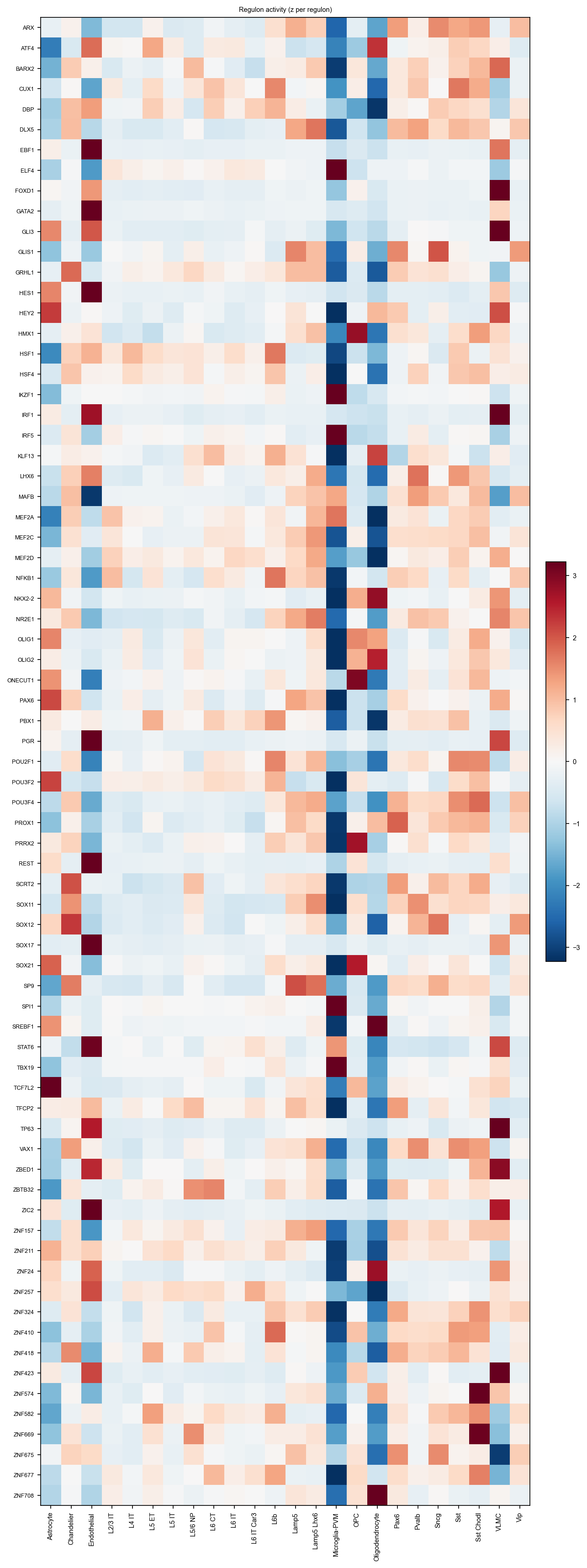

spec = cytorete.tl.regulonSpecificity(adata, groupby="Subclass", copy=True)
cytorete.pl.regulonSpecificityScatter(adata, groupby="Subclass",
                                      key="X_regulon")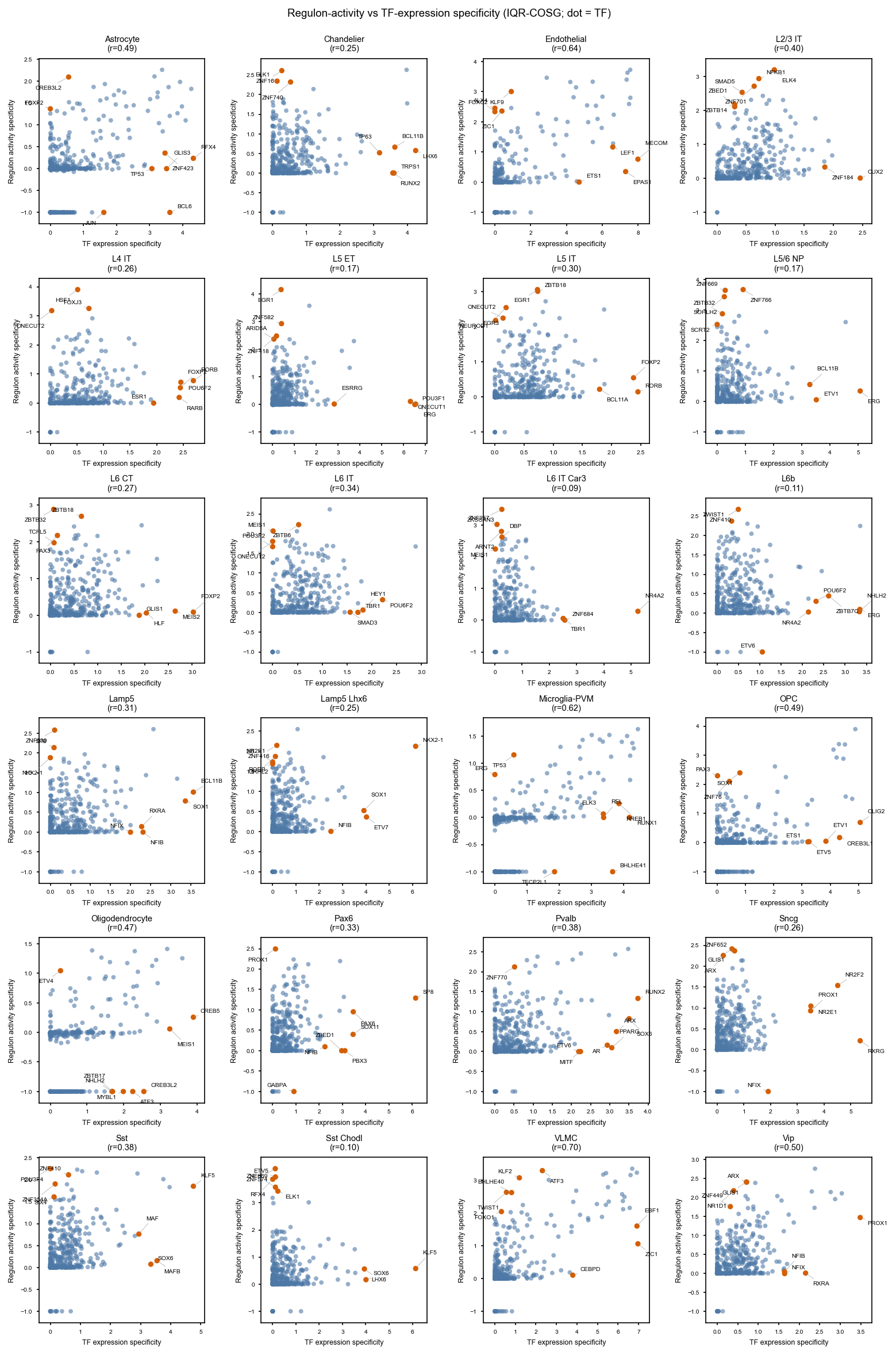

key="X_regulon" is needed here as on the cytome page: the function defaults to "X_grn", which is inferGRN’s key rather than inferRegulon’s.

Activity on the embedding, using an ordinary obs column rather than a cytome cells column:

for tf in ["CUX2", "LHX6", "IRF8"]:
    adata.obs[f"act_{tf}"] = A[:, names.index(tf)]

piaso.pl.plotEmbedding(adata, color=[f"act_{t}" for t in ["CUX2", "LHX6", "IRF8"]],
                       basis="X_umap", vmin_pct=5, vmax_pct=95)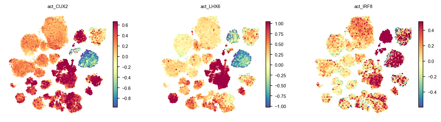

The per-cell p-values come with it: CUX2 clears p < 0.05 in 29% of cells, LHX6 in 20%, IRF8 in 4% — IRF8’s regulon is real and confined to microglia, which is a small fraction of this dataset, so few cells can individually beat their own control sets. Specificity and per-cell significance are different questions; §3b of the cytome page reads that distinction out in full.

Which container should you use?

Not this one, if the data is large. The chain here holds the matrix, the promoter sequences and the activity matrix in memory at once; on a .cytome every stage streams and peak memory is set by the batch size instead of by the cell count. Twenty thousand nuclei is comfortable either way, and an atlas is not.

Use an AnnData when the object is already in memory and you want one more result on it. Use a cytome when the object does not fit, or when you want the result to persist without re-running anything.

Related

• cytorete: RNA regulons — the same chain on a cytome, with the biology read out in full.
• Motif analysis — the motif engine underneath, and why a motif-only version of this analysis does not work.
• cytorete across development — regulon dynamics at half a million bins.