Gene set scoring: PIASOscore

piaso.tl.score answers “how much is this gene set on, in this cell”. The statistic it computes is the PIASOscore: the mean of the set minus the mean of control gene sets matched to it, plus a per-cell empirical p-value from those same controls.

The control sets are the whole point. A gene set’s raw mean expression is mostly a function of how deeply the cell was sequenced and how highly expressed its genes happen to be. This page measures that rather than asserting it.

import numpy as np
import pandas as pd
import anndata as ad
import piaso, cosg

piaso.settings.set_figure_params(style="cell")

1. Data

SEA-AD middle temporal gyrus, 20,000 nuclei, 24 annotated subclasses:

adata = piaso.data.load_dataset("sea_ad_mtg_20k")
adata.shape, list(adata.layers), list(adata.obsm)

((20000, 36601), ['UMIs'], ['X_scVI', 'X_umap'])

Check where the raw counts are before normalizing. On this dataset .X is already normalized and the integer UMIs live in a layer, so infog has to be told:

piaso.tl.infog(adata, layer="UMIs", n_top_genes=3000)

Passing layer= wrong is not a crash: it is a quieter, worse outcome. Running this page with the default .X still produced sensible-looking microglial scores; it just resolved them far less sharply (41% of microglia significant with the right layer, 32% with the wrong one). piaso.data.dataset_info() reports a counts_layer field where the dataset registry knows it.

2. One gene set

MICROGLIA = ["P2RY12", "CX3CR1", "CSF1R", "C1QA", "C1QB", "C1QC", "AIF1",
             "TMEM119", "TYROBP", "ITGAM", "PTPRC", "DOCK8", "APBB1IP",
             "SPI1", "IRF8", "MRC1", "CD74", "HLA-DRA"]

piaso.tl.score(adata, gene_list=MICROGLIA, key_added="microglia",
               compute_pvalues=True)

3.2 s for 20,000 cells. The score lands in adata.obs, the full statistics in adata.uns:

list(adata.uns["microglia"].columns)

['score', 'score_query', 'score_ctrl_average',
 'pval_mc', 'nlog10_pval_mc', 'pval_mc_FDR', 'nlog10_pval_mc_FDR',
 'pval', 'nlog10_pval', 'pval_FDR', 'nlog10_pval_FDR']

score_query is the set’s own mean, score_ctrl_average the mean of its control sets, and score is the difference. Two p-values are reported: pval_mc compares each cell against its own control sets (Monte Carlo), and pval is a pooled empirical p-value. Both come with a Benjamini–Hochberg FDR.

adata.obs.groupby("Subclass", observed=True)["microglia"].median().sort_values(
    ascending=False).head(4)

Microglia-PVM    13.18
...

The next-highest subclass is two orders of magnitude below. That is the answer you want, and now the part worth checking.

3. Why the control set exists

Compare against the obvious alternative — the plain mean of the same genes in the same normalized matrix:

idx = [adata.var_names.get_loc(g) for g in MICROGLIA]
naive = np.asarray(adata.layers["infog"][:, idx].mean(axis=1)).ravel()
adata.obs["microglia_mean"] = naive

depth = np.asarray(adata.layers["UMIs"].sum(axis=1)).ravel()
np.corrcoef(naive, np.log1p(depth))[0, 1], \
    np.corrcoef(adata.obs["microglia"], np.log1p(depth))[0, 1]

(-0.238, 0.010)

The naive mean carries a −0.24 correlation with sequencing depth. The PIASOscore carries 0.01 — depth is gone. That is what the control sets buy: they are drawn to match the query set’s expression profile, so whatever the query picks up from depth, the controls pick up too, and subtracting removes it.

Be honest about the cost:

mg = adata.obs["Subclass"] == "Microglia-PVM"
def separation(v):
    v = np.asarray(v, float)
    return (v[mg].mean() - v[~mg].mean()) / v.std()

separation(naive), separation(adata.obs["microglia"])

(5.27, 4.39)

The naive mean separates microglia slightly better — 5.3 SD against 4.4. If your only goal is to rank cells within one dataset, it is not obviously worse. The score’s advantage appears the moment you compare across cells of different depth, across samples, or across gene sets of different size, where the naive mean’s −0.24 is an artefact that travels with the number.

Side by side on the embedding, the two look much the same where it matters:

adata.obs["microglia_naive"] = naive

piaso.pl.embedding(adata, basis="X_umap",
                   color=["microglia", "microglia_naive"], ncol=1)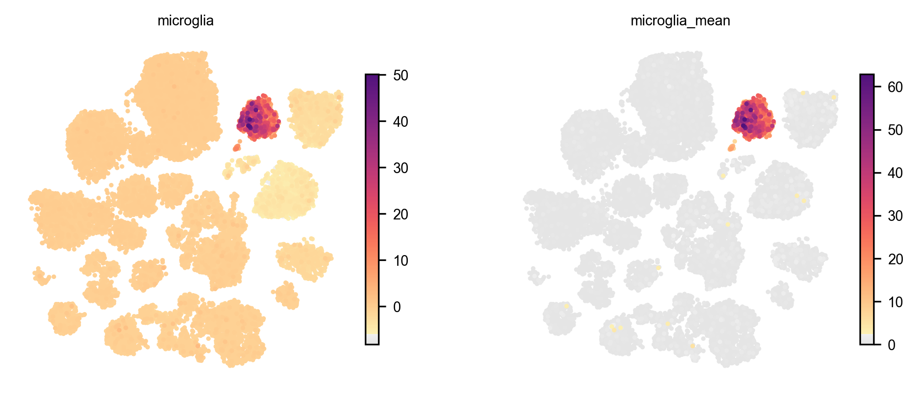

Both light up the same island, which is the point: the disagreement is not about which cells are microglia. It is that the naive panel’s values also track how deeply each cell was sequenced, so the same cell type scores differently in a shallow sample than a deep one — invisible here, and the reason the two panels stop agreeing the moment a second sample arrives.

Where the idea comes from, and what is ours

Scoring a gene set against matched control sets rather than against nothing is not new — it is the design in scDRS (Zhang et al., Nature Genetics 2022), and it is shared in spirit with AUCell and Vision. PIASOscore uses that construction (with per-gene nearest-neighbour matching where scDRS uses bins), and its empirical-null p-value follows the scDRS formulation: p = (1 + #{T_ctrl >= T}) / (1 + n_ctrl).

What is different is how the control sets are evaluated. The obvious implementation loops over control sets and subsets the matrix once per set, which costs O(nnz) each time, so the total grows linearly in the number of controls. PIASOscore packs every gene set and every one of its control sets into a single sparse weight matrix and evaluates them as one matrix multiplication per chunk, so the cost is nearly flat in the number of control sets instead of linear. Measured on this scoring path, loop versus matmul at 20 / 80 / 320 sets:

loop    1.95 s   6.45 s   24.41 s
matmul  0.55 s   0.62 s    0.78 s

That is what makes n_ctrl_set=100 — and a 1,000-set pathway database — routine rather than a decision you have to weigh. The null is the same null; what changed is how fast it is to compute.

What else differs from scDRS

Beyond the evaluation, four things:

	scDRS	PIASOscore
Control-set selection	matched on mean expression and variance, drawn from discretised bins (`n_mean_bin` × `n_var_bin`)	matched on the same two statistics, but as each gene’s k nearest neighbours in (mean, variance) space — a tighter per-gene match — and drawn against the scored layer so the controls and the query see identical normalisation
Normalisation	expects a normalised matrix and does not check	`layer=`/`score_layer=` are explicit, and INFOG refuses non-integer input rather than silently transforming twice
Execution	in-memory, one gene set at a time	one sparse matmul per chunk over all sets and controls, in a Rust kernel
Scale	the matrix must fit in RAM	streamed from a `.cytome`, so memory is set by chunk size and not by cell count

A head-to-head benchmark is in preparation for the manuscript; the numbers so far look good, and this page deliberately quotes only what is measured here — the timings above — rather than getting ahead of it. The code is public, so the design differences are checkable without waiting for us.

4. Per-cell p-values

sig = adata.uns["microglia"]["pval_mc"] < 0.01
sig.sum(), 100 * sig.mean()

(264, 1.32)

pd.crosstab(adata.obs["Subclass"], sig.values,
            normalize="index")[True].sort_values(ascending=False).head(3)

Microglia-PVM    0.412
Lamp5 Lhx6       0.003
Pax6             0.000

41% of microglia, 0.3% of the next subclass. The p-value is doing real work — it is a per-cell statement, not a group-level one, so it can be used as a gate: adata[sig] is the set of cells for which this programme is individually defensible.

Note that 41% is not 100%. Not every microglial nucleus in a snRNA-seq dataset has enough counts for an 18-gene set to clear p<0.01 against its own controls. Reporting the fraction, rather than the median score, is usually the more honest summary.

5. A whole pathway database at once

Pass a dict — or a DataFrame, or a list of lists — and every set is scored in a single batched pass:

import gseapy as gp
kegg = gp.parser.get_library("KEGG_2021_Human")
len(kegg)

score_matrix, names, pvals = piaso.tl.score(adata, gene_list=kegg)
score_matrix.shape

(20000, 320)

51.3 s for 320 gene sets × 20,000 cells: one hstacked sparse matmul rather than 320 separate ones, on the Rust backend. The return is a tuple here, not an in-place write, because there is no single key_added to write to.

6. Treat the scores as a matrix

The score matrix is cells × gene sets, which is the same shape as cells × genes. So every tool that works on expression works on it — including COSG, which then finds which pathway is a marker of which cell type:

adata_score = ad.AnnData(X=np.asarray(score_matrix),
                         obs=adata.obs.copy(),
                         var=pd.DataFrame(index=list(names)))
adata_score.obsm = adata.obsm.copy()

cosg.cosg(adata_score, key_added="cosg", groupby="Subclass",
          n_genes_user=5, mu=1, remove_lowly_expressed=False)
pd.DataFrame(adata_score.uns["cosg"]["names"]).head(3)

Microglia-PVM   : Yersinia infection; Fc gamma R-mediated phagocytosis;
                  NOD-like receptor signaling pathway
Oligodendrocyte : Ether lipid metabolism; Bacterial invasion of epithelial
                  cells; AMPK signaling pathway
Astrocyte       : Propanoate metabolism; Fatty acid biosynthesis;
                  PPAR signaling pathway
L2/3 IT         : Dopaminergic synapse; Phosphatidylinositol signaling
                  system; Amphetamine addiction
Pvalb           : Butanoate metabolism; Taurine and hypotaurine metabolism;
                  Thermogenesis

Read those with KEGG’s naming in mind. “Yersinia infection” and “Bacterial invasion of epithelial cells” are not statements about bacteria in this tissue: they are phagocytosis and cytoskeletal-remodelling gene sets that KEGG curated from infection studies. What the result actually says is: microglia score highest on phagocytosis and innate immune signalling, astrocytes on lipid and fatty-acid metabolism, excitatory neurons on synaptic signalling. Every one of those is right, and none of them was given to the method.

piaso.pl.embedding(adata_score, basis="X_umap",
                   color=["Lysosome", "Oxidative phosphorylation"])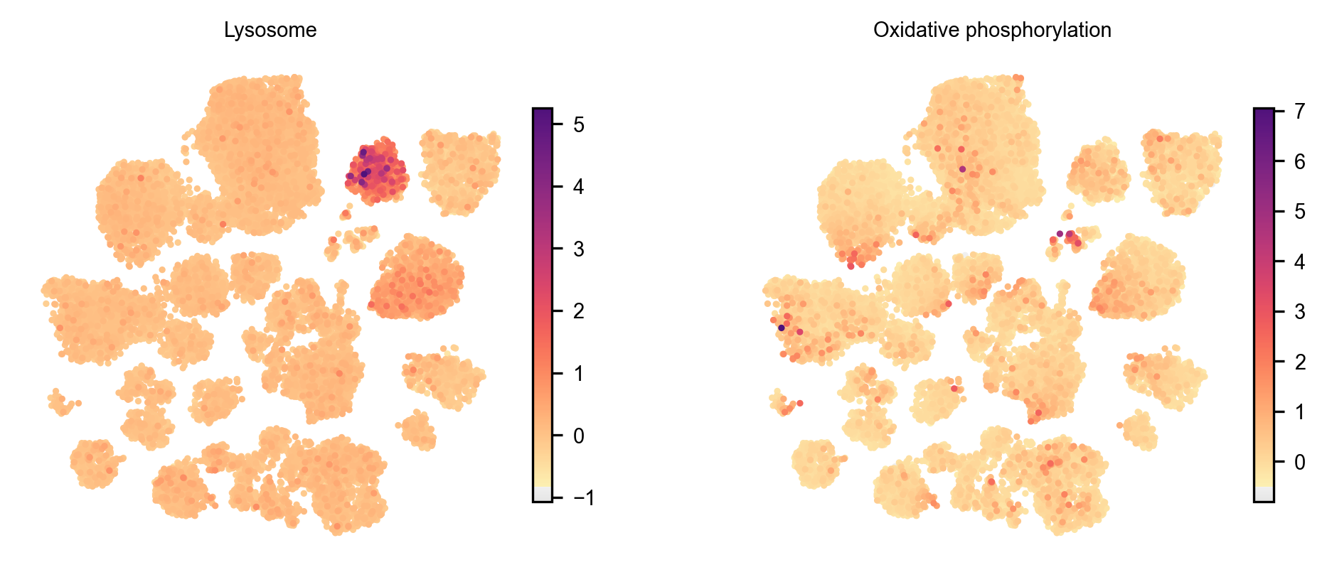

top = pd.DataFrame(adata_score.uns["cosg"]["names"])
selected = list(dict.fromkeys(g for c in top.columns for g in top[c].head(2)))
piaso.pl.dotplot(adata_score, selected, groupby="Subclass",
                 standard_scale="var")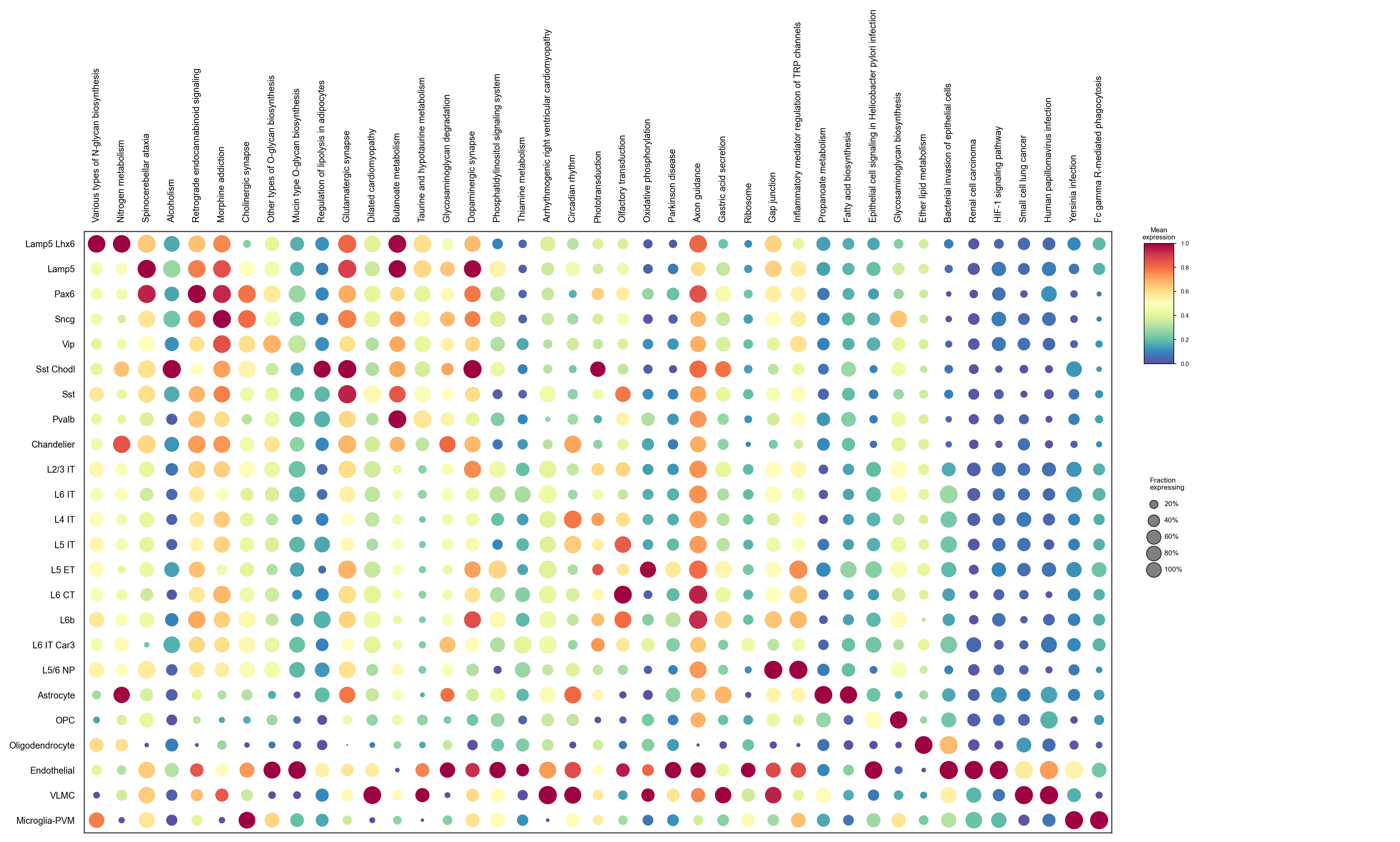

7. On a cytome

The same call takes a path to a .cytome file, and streams:

import cytome

ds = cytome.open("atlas.cytome")
piaso.tl.score(ds, gene_list=kegg, modality="RNA", batch_size=1024)

Peak memory is set by batch_size, not by the number of cells. For a single gene set with key_added, the score is written to ds.cells[key_added] and the p-value columns follow pvalue_to= ('cells', 'metadata', or 'both').

Parameters worth knowing

parameter	what it changes
`n_ctrl_set`	how many control sets per gene set (default 100). More is a tighter null and a slower run.
`n_nearest_neighbors`	how control genes are matched to query genes (default 30).
`gene_weights`	weight genes within a set — useful when the set comes with scores.
`compute_pvalues`	off by default in multi-set mode; p-values for hundreds of sets are expensive.
`layer`	which matrix to score. Defaults to `infog`.
`random_seed`	the control sets are sampled; fix it for reproducibility.

Where to go next

KEGG and ChEMBL gene sets: the same approach applied to drug-target sets, from the previous release.
Datasets and genome references: what piaso.data will fetch for you.