Xenium Prime 5K: a mouse brain hemisphere end to end

This page runs 10x Genomics’ public Xenium Prime 5K fresh-frozen mouse brain section from the raw output bundle to annotated clusters: 63,173 segmented cells × 5,006 genes, one coronal hemisphere.

Brain is the right tissue to learn a spatial workflow on, because the answer is already known. A coronal hemisphere has cortical layers, a hippocampus with a dentate gyrus, a striatum and a thalamus, arranged the same way in every mouse. So every step below can be checked against anatomy rather than taken on trust — and the last section does exactly that.

1. Getting the data without downloading 13 GB

The output bundle is a 13.3 GB ZIP. An analysis needs the cell-feature matrix and the cell table, which are 55 MB of it.

A ZIP stores its index at the end of the file, so with HTTP range requests you can list the archive and pull single members. Both 10x hosts support them:

import io, urllib.request, zipfile

URL = ("https://cf.10xgenomics.com/samples/xenium/3.0.0/"
       "Xenium_Prime_Mouse_Brain_Coronal_FF/"
       "Xenium_Prime_Mouse_Brain_Coronal_FF_outs.zip")

class HTTPRangeFile(io.RawIOBase):
    def __init__(self, url):
        self.url, self._pos = url, 0
        self.size = int(self._get(0, 0, head=True))
    def _get(self, start, end, head=False):
        req = urllib.request.Request(self.url, headers={
            "Range": f"bytes={start}-{end}",
            # cf.10xgenomics.com 403s urllib's default User-Agent
            "User-Agent": "Mozilla/5.0"})
        with urllib.request.urlopen(req, timeout=300) as r:
            return r.headers["Content-Range"].split("/")[1] if head else r.read()
    def seekable(self): return True
    def readable(self): return True
    def seek(self, off, whence=0):
        self._pos = (off if whence == 0 else self._pos + off
                     if whence == 1 else self.size + off)
        return self._pos
    def tell(self): return self._pos
    def read(self, n=-1):
        n = self.size - self._pos if n is None or n < 0 else min(n, self.size - self._pos)
        if n <= 0:
            return b""
        data = self._get(self._pos, self._pos + n - 1)
        self._pos += len(data)
        return data
    def readinto(self, b):
        data = self.read(len(b)); b[:len(data)] = data; return len(data)

zf = zipfile.ZipFile(io.BufferedReader(HTTPRangeFile(URL), 1 << 20))
for name in ("experiment.xenium", "cells.parquet", "cell_feature_matrix.h5",
             "analysis.tar.gz"):
    with zf.open(name) as src, open(name, "wb") as dst:
        dst.write(src.read())

That is 83 MB instead of 13.3 GB, and it takes seconds. Add morphology_focus/morphology_focus_0000.ome.tif (376 MB) if you want the image overlay from the other Xenium tutorial.

experiment.xenium is a small JSON worth reading first:

import json
meta = json.load(open("experiment.xenium"))
meta["run_name"], meta["panel_name"], meta["panel_num_targets_predesigned"]

('Mouse FF Brain Hemisphere (Coronal) 5K',
 'Xenium Mouse 5K Pan Tissue & Pathways Panel', 5006)

2. Loading it

Newer Xenium runs write cells.parquet rather than cells.csv.gz; the columns are the same.

import numpy as np
import pandas as pd
import piaso, cosg

piaso.settings.set_figure_params()

adata = piaso.pp.read_10x_h5("cell_feature_matrix.h5")
adata.var_names_make_unique()

cells = pd.read_parquet("cells.parquet")
cells["cell_id"] = cells["cell_id"].astype(str)
cells = cells.set_index("cell_id").loc[adata.obs_names]

adata.obsm["spatial"] = cells[["x_centroid", "y_centroid"]].to_numpy()   # microns
for col in ("transcript_counts", "control_probe_counts",
            "control_codeword_counts", "cell_area", "nucleus_area",
            "nucleus_count", "segmentation_method"):
    adata.obs[col] = cells[col].values

adata.shape, np.median(adata.obs["transcript_counts"])

((63173, 5006), 1088.0)

1,088 transcripts per cell at the median. That is the number that makes this dataset behave like scRNA-seq rather than like a 300-plex panel, where a few hundred is normal.

3. QC, including the part that is specific to Xenium

Two of the three panels below are the usual ones. The third is not available in scRNA-seq at all.

The panel carries negative-control probes and codewords — sequences that match nothing in the transcriptome, plus codewords that decode to nothing. They cannot produce a real signal, so their rate is a direct measurement of the background, not an estimate from the data.

ctrl = adata.obs["control_probe_counts"] + adata.obs["control_codeword_counts"]
total = adata.obs["transcript_counts"] + ctrl
100 * ctrl.sum() / total.sum()

0.007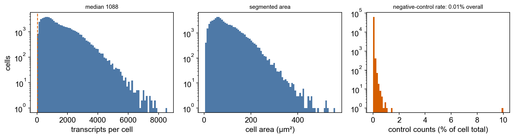

Transcripts per cell, segmented area, and the negative-control rate

0.007% of all counts are controls. That is the false-detection floor for this run, and it is low enough that a gene detected in a handful of cells is not obviously noise. On a run where this came back at 1–2%, every downstream threshold would need to account for it — which is the reason to look before clustering rather than after.

segmentation_method is worth a glance too:

Segmented by interior stain (18S)                      59317
Segmented by nucleus expansion of 5.0µm                 3250
Segmented by boundary stain (ATP1A1+CD45+E-Cadherin)     606

The 3,250 cells segmented by nucleus expansion are the ones where the stain gave no boundary and the pipeline drew a 5 µm circle instead. They are not wrong, but their transcripts are assigned by geometry rather than by morphology, so if a result rests on those cells specifically, check it.

adata = adata[(adata.obs["transcript_counts"] >= 25)
              & (adata.obs["cell_area"] > 0)].copy()
adata.layers["counts"] = adata.X.copy()
adata.shape

(63125, 5006)

Only 48 cells go. Xenium’s segmentation already dropped the debris; the filter is here to catch what it missed, not to do the work.

4. INFOG + GDR as the dimensionality reduction

Nothing here is spatial. The matrix is a matrix.

The embedding this page uses is INFOG followed by GDR. The SVD in the middle is scaffolding, not the destination: GDR builds its axes on marker-gene structure, so it needs a preliminary grouping to compute markers for, and a quick SVD-based clustering is the cheapest way to get one.

# 1. INFOG: normalisation that keeps count structure
piaso.tl.infog(adata, layer="counts", n_top_genes=3000, key_added="infog")

# 2. a preliminary grouping, only so GDR has something to build axes on
piaso.tl.runSVD(adata, layer="infog", n_components=50, key_added="X_svd",
                scale_data=False)
piaso.tl.neighbors(adata, use_rep="X_svd", n_neighbors=15)
piaso.tl.leiden(adata, resolution=1.0, key_added="leiden_prelim")

# 3. GDR: one dimension per preliminary group, built on its marker genes
piaso.tl.runGDR(adata, groupby="leiden_prelim", layer="infog",
                score_layer="infog", n_gene=30, mu=10.0)

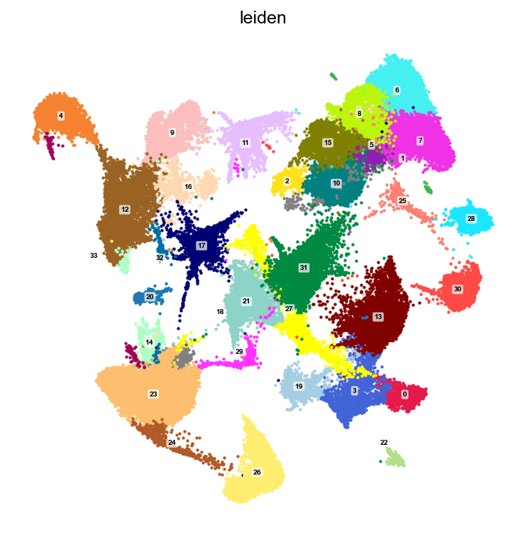
# 4. everything downstream lives in the GDR space
piaso.tl.neighbors(adata, use_rep="X_gdr", n_neighbors=15)
piaso.tl.leiden(adata, resolution=1.0, key_added="leiden")
piaso.tl.umap(adata, use_rep="X_gdr")

INFOG takes 1.4 s and GDR 3.9 s; the whole sequence is under two minutes on 63,125 cells.

X_gdr has 38 dimensions — one per preliminary cluster, not 50 arbitrary components. That is the practical difference from an SVD: every axis is “how much does this cell look like preliminary group k”, so the space is interpretable, and the number of dimensions is set by the data rather than chosen.

Re-clustering in that space gives 34 clusters from the 38 it started with, and it is not merely a relabelling of the input — ARI 0.60, NMI 0.76 against the preliminary clustering. GDR pulls apart groups that the SVD had split on variance rather than identity, and merges ones that differed by depth of sequencing rather than by cell type.

On a panel dataset this matters more than on whole-transcriptome data: 5,006 genes chosen for cell-type discrimination are already close to a marker panel, which is exactly the structure GDR is built to use.

5. Markers

adata.X = adata.layers["infog"]
cosg.cosg(adata, groupby="leiden", key_added="cosg", mu=100, n_genes_user=30,
          calculate_pvalues=True)
pd.DataFrame(adata.uns["cosg"]["names"]).iloc[:5, :8]

Six and a half seconds. Reading the first few clusters straight off:

cluster	top markers	reading
5	Sst, Crhbp, Six3, Lhx6, Cort	SST interneurons
7	Pvalb, Syt2, Oprd1, Kcnab3	PV interneurons
6	Nptxr, Igfn1, Lamp5, Cacng3	LAMP5 interneurons
3	Tagln, Myh11, Pln, Gja5, Eln	vascular smooth muscle
0	Slc47a1, Bnc2, Sphk1, Foxc2, Msln	meninges

The interneuron classes come out separated and named by their canonical genes, without any reference being consulted. See the COSG tutorial for what mu and the p-value columns do.

6. The check: does the map match the brain?

This is the section that makes brain a good teaching dataset. Plot canonical genes back into tissue space and see whether they land where anatomy says they should.

adata.X = adata.layers["counts"].copy()
piaso.pp.normalize_log1p(adata)

genes = ["Slc17a7", "Cux2", "Rorb", "Fezf2", "Foxp2", "Gad1",
         "Prox1", "Mog", "Aqp4", "Folr1", "Pdgfra", "Cx3cr1"]
piaso.pl.embedding(adata, color=genes, basis="spatial", point_size=0.55,
                   ncols=5, fix_coordinate_ratio=True)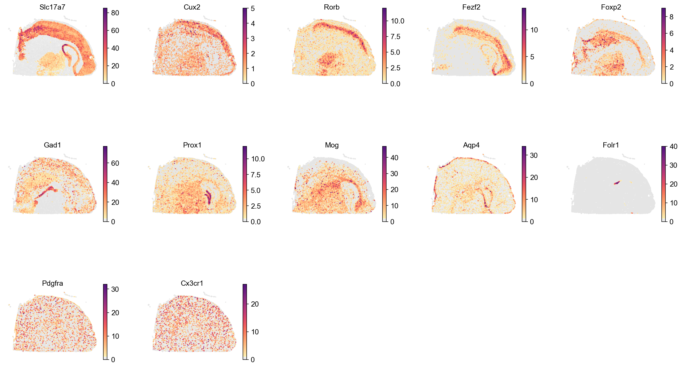

Every panel is checkable:

Cux2 → Rorb → Fezf2 → Foxp2 walk down the cortical layers, L2/3 to L6, as four bands at increasing depth from the surface. Getting this gradient in the right order is the single strongest sign the coordinates, the segmentation and the normalisation are all sound.
Prox1 draws the dentate gyrus as a sharp arc — one of the most recognisable structures in the brain, and one no clustering was told about.
Slc17a7 (excitatory) fills cortex and hippocampus and stops at the striatum; Gad1 (inhibitory) does the opposite.
Aqp4 is strongest at the pial surface and along vessels, which is where astrocyte endfeet are.
Pdgfra (OPCs) and Cx3cr1 (microglia) are scattered evenly, as they should be — a uniform pattern is a positive result for those two, and would be a red flag for a layer marker.

fix_coordinate_ratio=True matters here: a section plotted with a stretched aspect ratio is a section you cannot compare with an atlas.

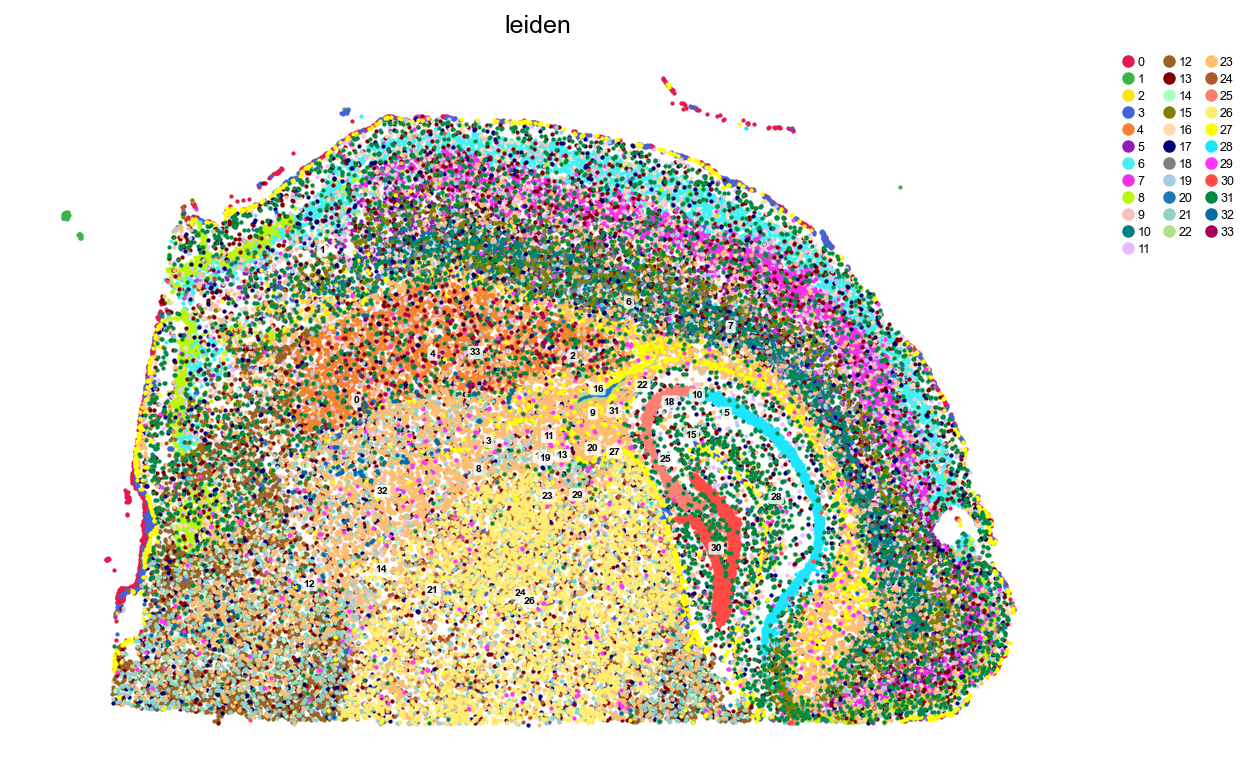
The clusters reproduce the same anatomy — layered bands in the cortex, the hippocampal arc with the dentate inside it, striatum and thalamus as large distinct territories — from expression alone.

A 5,006-gene panel is still a panel

Worth knowing before you plan an experiment around one:

[g for g in ("Mbp", "Plp1", "Ttr", "Cldn5") if g not in adata.var_names]

['Mbp', 'Plp1', 'Ttr', 'Cldn5']

Mbp and Plp1 — the two genes most people name first for oligodendrocytes — are not on this panel. Neither is Ttr for choroid plexus, nor Cldn5 for endothelium. The panel covers those cell types perfectly well through other genes (Mog and Sox10 for oligodendrocytes, Folr1 for choroid plexus), so nothing is lost; but a script that hard-codes a favourite marker will fail on a panel dataset, and the failure looks like “this cell type is absent”.

Check membership before you plan, not after you plot. The Atera WTA tutorial is the version of this problem where it does not arise.

7. Cell types from PIASOmarkerDB, and whether they are right

Clusters are not cell types until someone names them. Rather than hand-annotate 34 clusters, take the naming from a reference: PIASOmarkerDB carries the Allen whole-mouse-brain taxonomy, so the names and their markers come from a study that never saw this section.

neuron_df, neuron = piaso.tl.getMarkers(
    study="AllenWholeMouseBrain_Neuron", as_dict=True)
nonneuron_df, nonneuron = piaso.tl.getMarkers(
    study="AllenWholeMouseBrain_NonNeuron", as_dict=True)

marker_sets = {**neuron, **nonneuron}
len(neuron), len(nonneuron), len(marker_sets)

(315, 26, 334)

315 neuronal and 26 non-neuronal types, 50 markers each, combining to 334 — seven names appear in both studies and the dictionary merge keeps one copy.

The panel does not carry every marker, so check the overlap before predicting:

panel = set(adata.var_names)
on_panel = {k: [g for g in v if g in panel] for k, v in marker_sets.items()}
kept = {k: v for k, v in on_panel.items() if len(v) >= 5}
len(kept), np.median([len(v) for v in on_panel.values()])

(334, 18.0)

The median type keeps 18 of its 50 markers, and all 334 keep at least five. A 5,006-gene panel designed for pan-tissue use covers a whole-brain taxonomy better than you might expect.

piaso.tl.predictCellTypeByMarker(
    adata, marker_gene_set=kept, score_method="piaso", score_layer="infog",
    use_rep="X_gdr", smooth_prediction=True, k_nearest_neighbors=7,
    key_added="CellTypes_markerdb")

35 seconds. Each cell is scored against all 334 marker sets, assigned the best, and then smoothed over its 7 nearest neighbours in the GDR space — which is the second reason the GDR step earlier was worth taking, since smoothing in a space built on marker structure is smoothing along the right axis.

adata.obs["CellTypes_markerdb"].value_counts().head(8)

327 Oligo NN                 9037
333 Endo NN                  4662
319 Astro-TE NN              3099
318 Astro-NT NN              2879
007 L2/3 IT CTX Glut         2850
151 TH Prkcd Grin2c Glut     2583
006 L4/5 IT CTX Glut         2363
334 Microglia NN             2123

223 of the 334 types are used. The rest are absent, which is correct: the Allen taxonomy covers the whole brain — cerebellum, medulla, olfactory bulb — and this is one coronal forebrain hemisphere.

Prediction across the section, 24 most abundant types

Is it right?

Names are cheap. The way to find out is to highlight types whose location is known in advance and look.

for cell_type in ["037 DG Glut", "007 L2/3 IT CTX Glut", "030 L6 CT CTX Glut",
                  "327 Oligo NN", "319 Astro-TE NN", "318 Astro-NT NN",
                  "151 TH Prkcd Grin2c Glut", "334 Microglia NN"]:
    piaso.pl.embedding(adata, color="CellTypes_markerdb", basis="spatial",
                       groups=[cell_type], na_color="0.92", point_size=0.8,
                       legend_loc="none", fix_coordinate_ratio=True)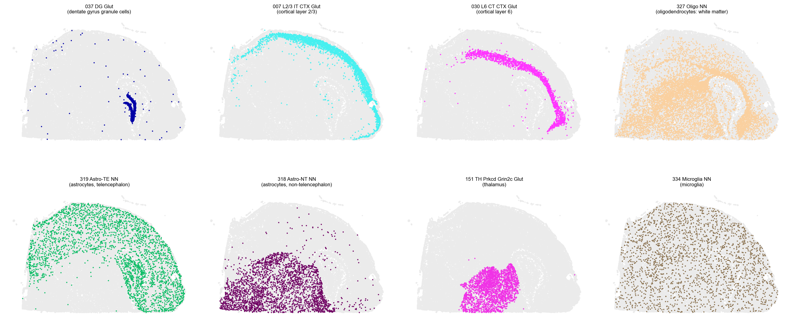

Eight predicted types highlighted in tissue space

Every panel is a test that could have failed:

037 DG Glut lands on the dentate gyrus, and only there — the V-shaped blade inside the hippocampal arc.
007 L2/3 IT CTX and 030 L6 CT CTX form two parallel bands, the first at the cortical surface and the second deep to it, in the right order.
327 Oligo NN fills the white-matter tracts — corpus callosum, internal capsule — and thins out in grey matter.
334 Microglia NN is scattered uniformly, which for microglia is the correct answer and would be a red flag for anything laminar.

The strongest one is the pair in the middle. The Allen taxonomy splits astrocytes by developmental origin — TE for telencephalon, NT for non-telencephalon — a distinction with no morphological signature, which nothing in this analysis was told about. Measuring the share of each inside the thalamic territory (defined independently by where the thalamic neuron types land):

type	share inside the thalamic territory
319 Astro-TE NN	0.2%
318 Astro-NT NN	29.5%

A 150-fold difference, in the direction embryology predicts. The prediction respects the telencephalon/diencephalon boundary, from marker genes alone.

That is the check to run on your own data: pick the types whose location you already know, highlight them one at a time, and only then trust the ones you did not.

8. Against 10x’s own clustering

The bundle ships 10x’s graph clustering in analysis.tar.gz, which makes a free sanity check.

import tarfile
with tarfile.open("analysis.tar.gz") as tf:
    m = next(m for m in tf.getmembers()
             if m.name.endswith("gene_expression_graphclust/clusters.csv"))
    tenx = pd.read_csv(tf.extractfile(m)).set_index("Barcode")["Cluster"]

from sklearn.metrics import adjusted_rand_score, normalized_mutual_info_score
adjusted_rand_score(adata.obs["leiden"], tenx.loc[adata.obs_names]), \
normalized_mutual_info_score(adata.obs["leiden"], tenx.loc[adata.obs_names])

(0.529, 0.685)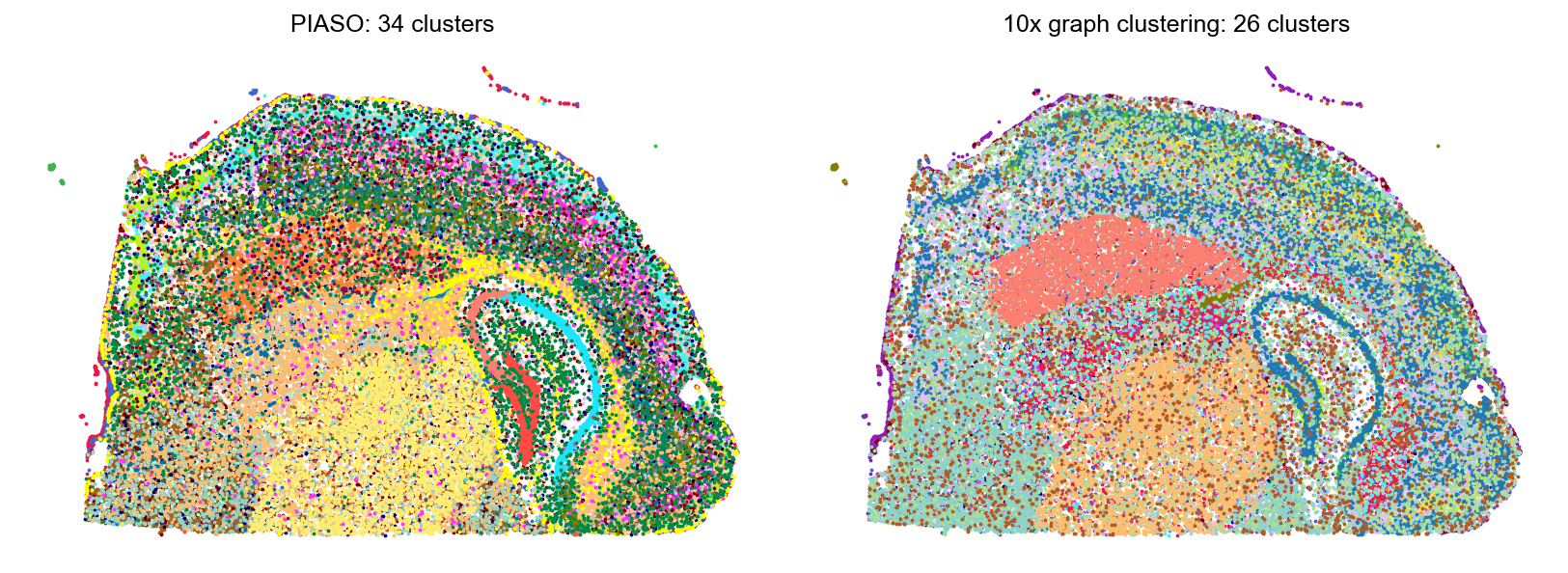

PIASO clusters against 10x's graph clustering, in tissue space

ARI 0.53, NMI 0.69, at 34 clusters against 10x’s 26. Read that as agreement on structure and disagreement on resolution, not as a disagreement about the biology: ARI punishes a split heavily even when the split is real, and 34 against 26 means several of 10x’s clusters are being divided. The tissue plot is the honest comparison — the same territories, drawn at different grain.

Worth noting against §4: clustering in the GDR space agrees with 10x better than the SVD-only clustering did (ARI 0.53 against 0.43). Two pipelines that share no code arriving closer together when one of them is built on marker structure is weak evidence, but it points the right way.

Which resolution you want depends on the question. For “where is the hippocampus”, 26 is plenty. For separating SST from PV interneurons, it is not.

Where to go next

Atera WTA — the same workflow on a different platform, with all 18,028 genes instead of a panel, and what that changes.
Xenium with tissue-image overlay — the morphology image, and selecting a region of interest.
Xenium into a cytome directly — for sections too large to hold in memory.
COSG markers — the marker step in full.
PIASOmarkerDB — the marker database used above, and the other 34 studies in it.
Downstream on Xenium — pathways, ligand–receptor and regulons on both sections.