
Downstream in situ: pathways, ligand–receptor and regulons
Clustering and markers are the start. The analyses that follow — pathway activity per cell, ligand–receptor signalling, transcription-factor regulons — all ask more of the gene list, and on targeted spatial data the panel decides in advance which of them are possible.
This page runs three of them on the two sections built in the other in-situ tutorials — one Xenium, one Atera, and opens with the measurement that should come first.
1. Check coverage before choosing an analysis
A ligand–receptor analysis needs both partners measured. A pathway score needs enough of the pathway’s genes. A regulon needs the transcription factor and its targets. None of that is guaranteed on a panel, and the failure is quiet: the analysis runs and returns a shorter answer.
So measure it first. Using the CellChat pairs that ship with LARIS:
import laris
lr = laris.datasets.lrDatabase(species="human")pairs = lr[["ligand", "receptor"]].dropna().drop_duplicates()
genes = set(adata.var_names)complete = pairs.apply(    lambda r: r.ligand in genes              and all(x.strip() in genes for x in str(r.receptor).split(",")),    axis=1)complete.sum(), len(pairs)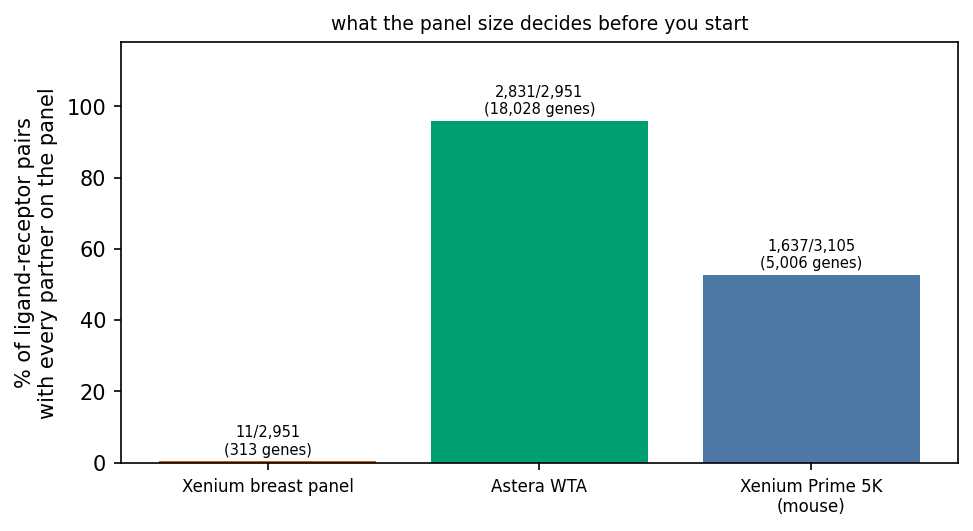
| panel | genes | complete L–R pairs | |
|---|---|---|---|
| Xenium human breast | 313 | 11 / 2,951 | 0.4% |
| Xenium Prime 5K (mouse) | 5,006 | 1,637 / 3,105 | 52.7% |
| Atera WTA | 18,028 | 2,831 / 2,951 | 95.9% |
This is the single most useful number to compute before planning a spatial experiment, and it is not linear in panel size. Going from 313 to 5,006 genes — 16× — takes L–R coverage from 0.4% to 52.7%, a 150× improvement, because a pair needs both ends and the probability of having both rises far faster than the gene count. Going from 5,006 to 18,028 takes it to 95.9%.
On a 313-gene panel, ligand–receptor analysis is not an option: eleven usable pairs is not a screen. It is a perfectly good panel for identifying cell types in breast tissue — it simply cannot answer this question, and the honest move is to know that before running the experiment rather than after.
2. KEGG pathways, scored per cell
piaso.tl.score scores a gene set per cell against matched control sets, so
the result is comparable across cells and across sets of different sizes. Given
a whole pathway library it produces a cells × pathways matrix that behaves like
an expression matrix — which means everything downstream (COSG, clustering,
spatial plotting) works on it unchanged.
import gseapy as gp
sets = gp.parser.get_library("KEGG_2019_Mouse")     # or KEGG_2021_Human
# Enrichr's mouse libraries carry HUMAN-cased symbols (CUX2) while a mouse# matrix uses title case (Cux2). Matching literally scores 1 set out of 300,# and looks like an empty result rather than a naming mismatch.by_upper = {}for name in adata.var_names:    by_upper.setdefault(str(name).upper(), str(name))sets = {k: sorted({by_upper[g.upper()] for g in v if g.upper() in by_upper})        for k, v in sets.items()}sets = {k: v for k, v in sets.items() if len(v) >= 5}
matrix, names, _ = piaso.tl.score(adata, gene_list=sets, layer="infog")
277 of ~300 mouse pathways are scorable on the 5,006-gene panel, and 319 of the human library on Atera. That case-folding step is worth keeping: it is the difference between 1 pathway and 277.
18 seconds for 277 pathways × 63,125 cells.
scored = ad.AnnData(X=np.asarray(matrix), obs=adata.obs.copy(),                    var=pd.DataFrame(index=list(names)))scored.obsm["spatial"] = adata.obsm["spatial"]
piaso.pl.embedding(scored, color=["Dopaminergic synapse", "Synaptic vesicle cycle",                                  "Oxidative phosphorylation",                                  "Antigen processing and presentation",                                  "ECM-receptor interaction",                                  "Complement and coagulation cascades"],                   basis="spatial", ncols=3, cmap="Spectral_r",                   vmin_pct=2, vmax_pct=98, fix_coordinate_ratio=True)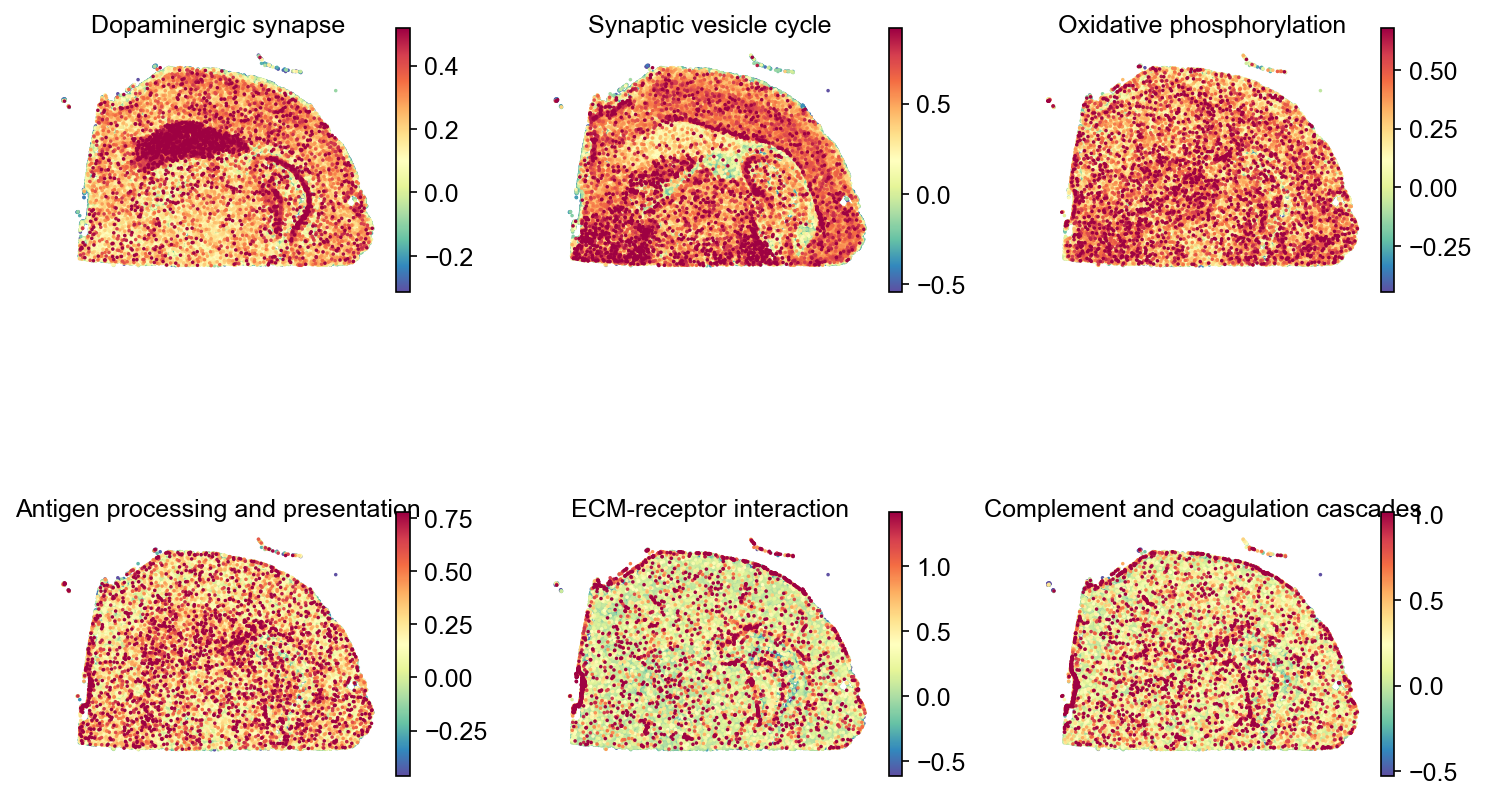
Two of these are checkable against anatomy, which is the reason to run it on brain first:
- Dopaminergic synapse picks out the striatum as a solid block. The caudoputamen is the densest dopaminergic target in the forebrain, and no step in this analysis was told where it is.
- ECM-receptor interaction and complement and coagulation both draw the pial surface and the vasculature — a thin rim and a branching network, which is where basement membrane and blood are.
- Antigen processing is scattered (microglia) with the same vascular rim.
- Synaptic vesicle cycle fills the neuropil-rich cortex and hippocampus and drops in white matter.
vmin_pct / vmax_pct are doing real work here: a few cells with extreme
scores otherwise flatten the entire section to one colour.
The same matrix answers “which pathway is specific to which cell type” by running COSG on it — see gene set scoring and KEGG and drug targets, where that idea is the whole page.
3. Ligand–receptor with LARIS
LARIS computes ligand–receptor interaction using the coordinates: a signal counts when the ligand-expressing cell and the receptor-expressing cell are actually near each other. That is the analysis spatial data exists for, and §1 is the reason it belongs on the WTA section rather than the panel one.
import laris
adata.obsm["X_spatial"] = np.asarray(adata.obsm["spatial"], dtype=np.float64)lr_df = laris.datasets.lrDatabase(species="human")
lr_data = laris.tl.prepareLRInteraction(    adata, lr_df=lr_df, number_nearest_neighbors=20,    use_rep_spatial="X_spatial")
laris.tl.runLARIS(lr_data, adata, use_rep="X_spatial",                  groupby="leiden", by_celltype=True,                  use_rep_spatial="X_spatial", n_top_lr=2000)
prepareLRInteraction builds the neighbourhood-weighted interaction matrix —
2,831 pairs on Atera and 1,637 on the mouse brain, the same numbers §1
predicted, which is the check that the coverage calculation and the tool agree.
Group by the clusters, not by the 223 predicted Allen types: LARIS tests every sender–receiver combination, so 223 types is ~50,000 of them against 34 clusters’ 1,156. That difference is hours against ninety seconds, and the extra resolution shows nothing the cluster-level answer does not.
| pairs | sender–receiver groups | time | significant at FDR < 0.05 | |
|---|---|---|---|---|
| Atera WTA (27 clusters) | 2,831 | 729 | 80 s | 14,548 |
| Mouse brain (34 clusters) | 1,637 | 1,156 | 92 s | 22,090 |
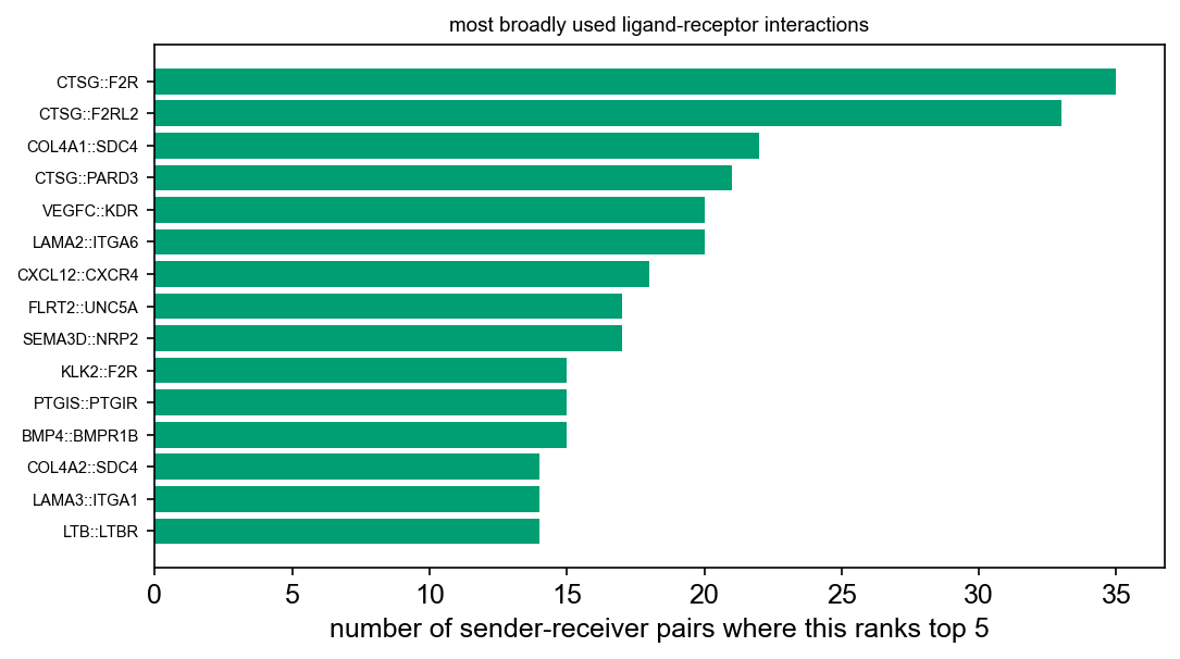
The interactions that rank top-5 in the most sender–receiver pairs are the ones worth reading first, and on both sections they are recognisable:
Breast tumour — CTSG::F2R and CTSG::F2RL2 (cathepsin G activating
protease-activated receptors), COL4A1::SDC4 and LAMA2::ITGA6 (basement
membrane to integrin/syndecan), CXCL12::CXCR4 and VEGFC::KDR.
The last two are the ones to notice. CXCL12–CXCR4 is the canonical chemokine
axis of breast cancer invasion and metastatic homing; VEGFC–KDR is
lymphangiogenic signalling, and the clusters section already found a distinct
lymphatic endothelial population by MMRN1/CCL21. Two independent parts
of the analysis pointing at the same biology is the kind of agreement worth
more than either alone.
Mouse brain — Dio3::Thra and Dio3::Thrb (deiodinase 3 with the thyroid
hormone receptors, the local control of thyroid signalling in brain), then
Slc17a7::Grik3, Slc17a7::Grm3 and Slc1a1::Grik3.
Those last three are glutamatergic synaptic signalling — the vesicular glutamate transporter and the glutamate transporter against kainate and metabotropic receptors. LARIS’s database carries neurotransmitter pairs as well as classical ligand–receptor ones, and on a brain section they come out on top, which is what they should do.
The score, in space
A ranked table is not what LARIS is for. The score is attached to a cell, so it can be drawn on the section — and that is the output worth looking at:
laris.pl.plotCCCSpatial(lr_data, basis="X_spatial", interaction="Slc17a7::Grik3", color_by="score", # 'cell_type' is the default size=6, fig_width=7)color_by="score" is the continuous per-cell overlay; the default colours by
cell type and requires one to be named.
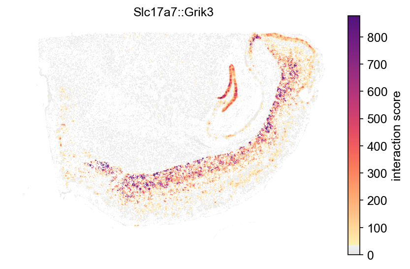
This is the one to check the method against. Slc17a7 is the vesicular
glutamate transporter and Grik3 a kainate receptor, so the interaction should
trace glutamatergic synaptic signalling — and it does: the hippocampal
pyramidal layer as a bright arc, the dentate gyrus as a hook inside it, the
cortical band around the outside, and essentially nothing in the striatum and
thalamus. No step in this analysis was told where the hippocampus is.
On the tumour section the same call gives a very different texture:
laris.pl.plotCCCSpatial(lr_data, basis="X_spatial", interaction="CTSG::F2R", color_by="score", size=6, fig_width=7)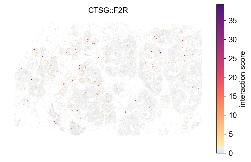
CTSG is cathepsin G, a mast-cell and neutrophil protease, and F2R is
PAR-1. The signal is punctate rather than laminar — scattered hot cells
against a cold background — which is what a rare secreting population acting
on its immediate neighbours looks like, and is consistent with the mast-cell
cluster the Atera page finds by CPA3 and
MS4A2.
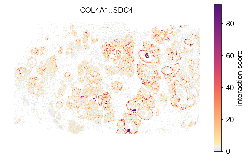
The contrast between those two panels is the argument for doing this in space at all: the same statistic, on two sections, describing a continuous anatomical sheet in one and a scatter of local events in the other. A sender–receiver table would have reported both as a number.
COL4A1::SDC4 — basement-membrane collagen against a syndecan — is the third
texture: neither laminar nor punctate but outlining structures, which is where
basement membrane is.
Note that 22,090 significant interactions is not 22,090 findings. It is a screen over 1.9 million combinations; the FDR controls the false-discovery proportion, and the list is a starting point to be read with the tissue in front of you, not a result set.
4. Regulons with cytorete
cytorete’s inferRegulon is the RNA-only
path — a SCENIC analogue built on COSG specificity plus promoter motif
scanning, so it needs no ATAC. It does need the genome and a motif database:
import cytorete, piaso
piaso.data.fetch_2bit("hg38")      # cached under ~/.piasopiaso.data.fetch_jaspar()
cytorete.inferRegulon(adata, genome="hg38", groupby="leiden",                      motif_db="jaspar")
inferGRN — the multi-omic version — needs an ATAC modality and so does not
apply to Xenium; inferRegulon is the one to reach for on RNA-only spatial
data.
What it does, in order: take the genes’ promoters from the genome, scan them for TF motifs to get a candidate TF → target map, then keep the edges where the TF and the target are co-specific to the same cell types by COSG. Motif presence alone is far too permissive; the co-specificity step is what turns it into a regulon.
[inferRegulon] 3769 genes with promoters (5985 intervals)[cistrome] scanning 520 PWMs (476 TFs) × 5985 promoter sequences[cistrome] M = 476 TFs × 3769 genes, 144713 edges (8.07% density)| groups | regulons | median targets | time | |
|---|---|---|---|---|
| Mouse brain (mm10) | 89 | 277 | 121 | 4 min |
| Atera WTA (hg38) | 27 | 344 | 152 | 23 min |
The whole-transcriptome section yields more regulons from fewer groups, which is what you would expect: the limit is how many TFs and targets are on the panel, not how many cell types you have.
regulonSpecificity then answers which regulon belongs to which cell type —
COSG again, run on the cells × regulon activity matrix rather than on
expression. Note it returns a long table (cell_type, regulon,
cosg_score, rank), not a wide matrix.
The results are the check, and on the breast tumour they are clean:
| cluster | top regulons | reading |
|---|---|---|
| 10 | SOX17, MEF2C, ERG, EBF1 | endothelium — SOX17 and ERG are the canonical endothelial TFs |
| 12 | SPI1, TFEC, MAF, RELB | myeloid — SPI1 is PU.1 |
| 1 | TFCP2L1, SNAI2, ZNF667, HOXA10 | basal / myoepithelial — SNAI2 is Slug |
| 11 | NR2F2, MEOX2, HOXD9, TBX15 | mesenchymal / fibroblast |
None of those TFs were supplied; they were recovered from promoter motifs plus co-specificity. That the myeloid cluster gets PU.1 and the endothelial cluster gets SOX17/ERG is the sign the inference is working, and it agrees with the marker-based identities from the Atera page without sharing any of that evidence.
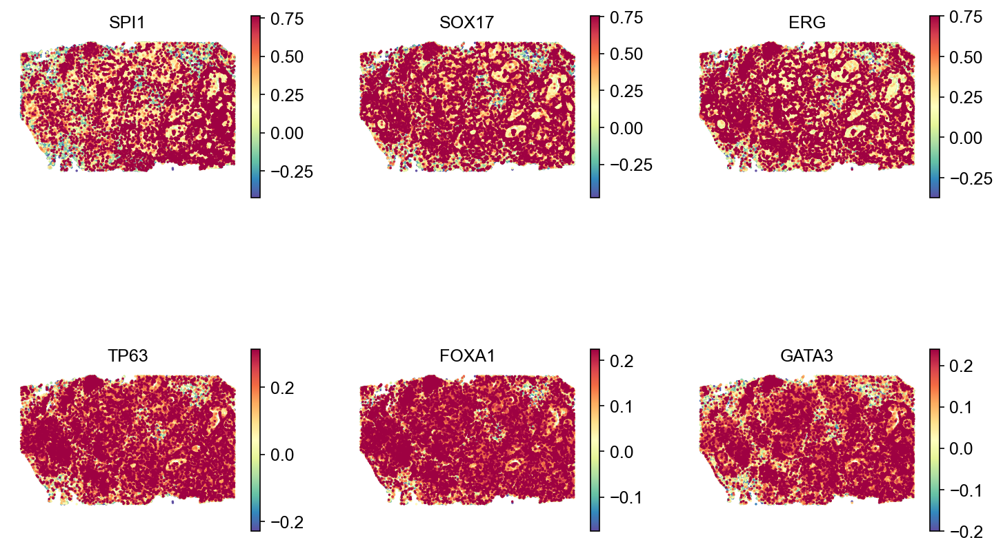
The way to check a regulon is to ask which cluster its activity peaks in, and whether that cluster’s marker genes — evidence the regulon inference never saw — agree:
| regulon | peak cluster’s markers | mean activity |
|---|---|---|
| SPI1 | CSF1R, CD14, MS4A7, C1QC | 1.03 |
| SOX17 | HBB, SEMA3G, GJA5, VEGFC | 0.99 |
| ERG | PLVAP, VWF, SLCO2A1, AQP1 | 0.84 |
| TP63 | TAT, KLK2, MUCL1, PADI4 | 0.20 |
| GATA3 | TAT, KLK2, MUCL1, PADI4 | 0.20 |
| FOXA1 | TAT, KLK2, MUCL1, PADI4 | 0.12 |
The top three are unambiguous. PU.1 (SPI1) peaks in the cluster marked by
CSF1R, CD14 and C1QC — macrophages, and PU.1 is the myeloid master
regulator. SOX17 and ERG, the two canonical endothelial factors, peak in
the two endothelial clusters (PLVAP/VWF vascular and SEMA3G/GJA5
arterial). Neither the TF nor the marker list was given to the other step.
The luminal factors are weaker and worth reading honestly: FOXA1, GATA3 and
TP63 all peak in the same luminal epithelial cluster (TAT, KLK2,
MUCL1), which is the right place, but at activities of 0.12–0.20 against
SPI1’s 1.03. A regulon with low activity spread over many similar clusters is a
weaker claim than one that spikes in a single population — the tumour
epithelium is most of this section and is split across several clusters, so the
specificity that COSG scores has little to grip. Read the number, not just
the ranking.
Group size decides whether this works
The mouse brain run is the cautionary half, and it is worth showing rather than omitting. Grouped by the 89 predicted Allen types with at least 50 cells — median group size 259 — the peaks are unstable:
| regulon | peak group | cells | peak among groups ≥ 500 cells |
|---|---|---|---|
| Spi1 | 334 Microglia NN | 2,123 | 334 Microglia NN |
| Tbr1 | 027 L6b EPd Glut | 478 | 007 L2/3 IT CTX Glut |
| Olig2 | 012 MEA Slc17a7 Glut | 127 | 319 Astro-TE NN |
| Sox9 | 142 HY Gnrh1 Glut | 53 | 333 Endo NN |
Spi1 → microglia is right and robust: PU.1, in the myeloid population, from a
group large enough to estimate. Tbr1 → L6b is right too — Tbr1 is a layer-6
identity factor — and stays in the cortical excitatory family when the small
groups are excluded.
Olig2 and Sox9 are not right. Both peak in groups of a hundred cells or
fewer, and both move to a different (more plausible, still not canonical)
population once a size floor is applied. That is the signature of an argmax
taken over many small groups: with 89 candidates of median 259 cells, some
group will score highest by noise.
So group by the coarsest labelling that still answers your question. The Atera run used 27 clusters of thousands of cells each and gave SPI1, SOX17 and ERG unambiguously; the brain run used 89 types of a few hundred and gave two right answers and two artefacts from the same pipeline. If you must use a fine taxonomy, impose a minimum group size and read the activity value, not just which group came first.
One practical note: this is the slowest analysis on the page — 23 minutes on the WTA section against 4 on the brain — because the cost is set by the number of genes whose promoters must be scanned, and the human run has far more of them.
Where to go next
- Xenium Prime 5K on mouse brain — where these objects are built.
- Atera WTA — the whole-transcriptome section.
- LARIS — the method, and comparisons across conditions.
- cytorete regulons — the regulon workflow in full.
- KEGG and drug targets — pathway and drug-set scoring as its own analysis.