GDR at scale: 200,000 cells in 17 minutes

runGDR builds a marker-gene-guided embedding. On a cytome it never loads the matrix: every stage streams chunks from the file, so the memory it needs is set by the chunk size and the worker count, not by the size of the dataset.

This page runs the whole thing on a 200,061-cell mouse developing visual cortex atlas — 35 libraries, 32,285 genes, 740 million nonzeros, 1.4 GB on disk — and reports what it costs. Timings are from a 20-core workstation.

The whole pipeline

import piaso

path = "allen_devvis_rna.cytome"

piaso.tl.infog(path, n_top_genes=3000, save_layer=True)
piaso.tl.runSVD(path, layer="infog", n_components=50, key_added="X_svd")

piaso.tl.runGDR(
    path,
    batch_key="library_prep",   # 35 libraries, each embedded on its own markers
    groupby=None,               # cluster within each batch rather than reuse labels
    n_gene=20,
    layer="infog",
    key_added="X_gdr",
    max_workers=8,
)

piaso.tl.neighbors(path, use_rep="X_gdr", n_neighbors=15, key_added="gdr")
piaso.tl.umap(path, use_rep="X_gdr", key_added="X_umap", neighbors_key="gdr")
piaso.settings.set_figure_params(style="cell")   # one house style across every figure

Nothing above returns a matrix. X_gdr (200,061 × 910) and X_umap are written into the cytome, so the next step reads them from disk.

What it looks like

piaso.pl.plotEmbedding(path, color="subclass_label", basis="X_umap")
piaso.pl.plotEmbedding(path, color="leiden_gdr",     basis="X_umap")
piaso.pl.plotEmbedding(path, color="library_prep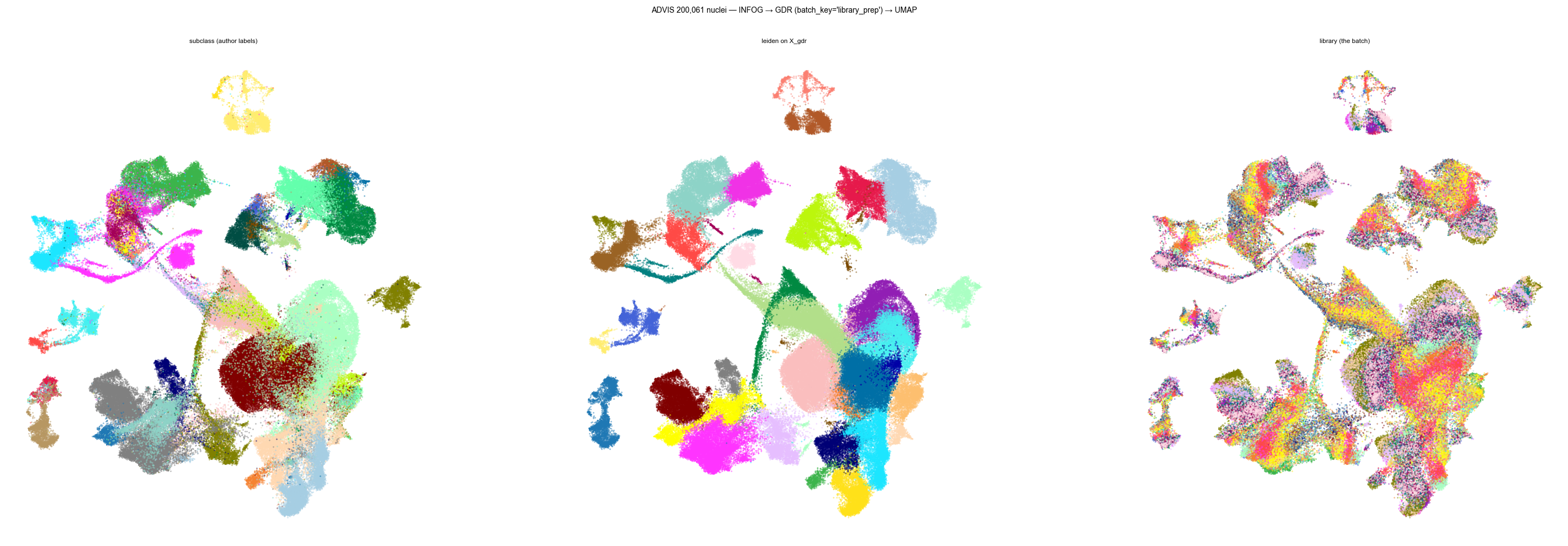",   basis="X_umap")

ADVIS 200k: subclass, Leiden on X_gdr, and the batch

Three colourings of one embedding, and the third is the one that makes the first two mean anything. The author subclass labels resolve into contiguous territories; Leiden run on X_gdr recovers them without being shown them; and library — the batch — is mixed evenly through every cluster rather than forming islands of its own.

That last panel is the check. GDR embedded each of the 35 libraries on its own markers, so batch structure is what it had the best opportunity to preserve. Colouring by subclass alone would look like success with nothing ruled out.

Subclass, at readable size

The three-panel figure above is a batch check, so its legends are suppressed. The same colouring on its own, with the labels:

piaso.pl.plotEmbedding(path, color="subclass_label", basis="X_umap")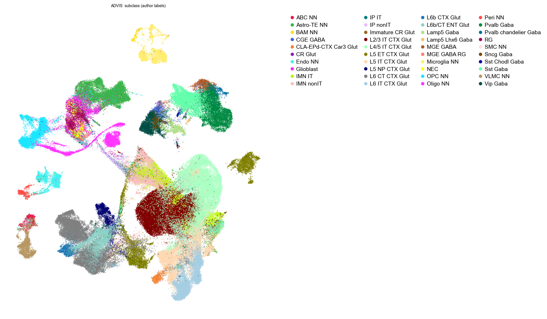

Biological variation survives the batch correction

batch_key="library_prep" mixed 35 libraries. The question that matters next is whether it also flattened the biology it was not asked about — this is a developmental dataset, and age is not the batch:

import re
ages = sorted(set(np.asarray(ds.cells["age_label"]).astype(str)),
              key=lambda a: (0 if a.startswith("E") else 1,
                             float(re.match(r"[EP](\d+(?:\.\d+)?)", a).group(1))))
ds.set_categories("age_label", order=ages)     # E before P, numeric within
piaso.pl.plotEmbedding(ds, color="age_label", basis="X_umap",
                       palette="Spectral_r")

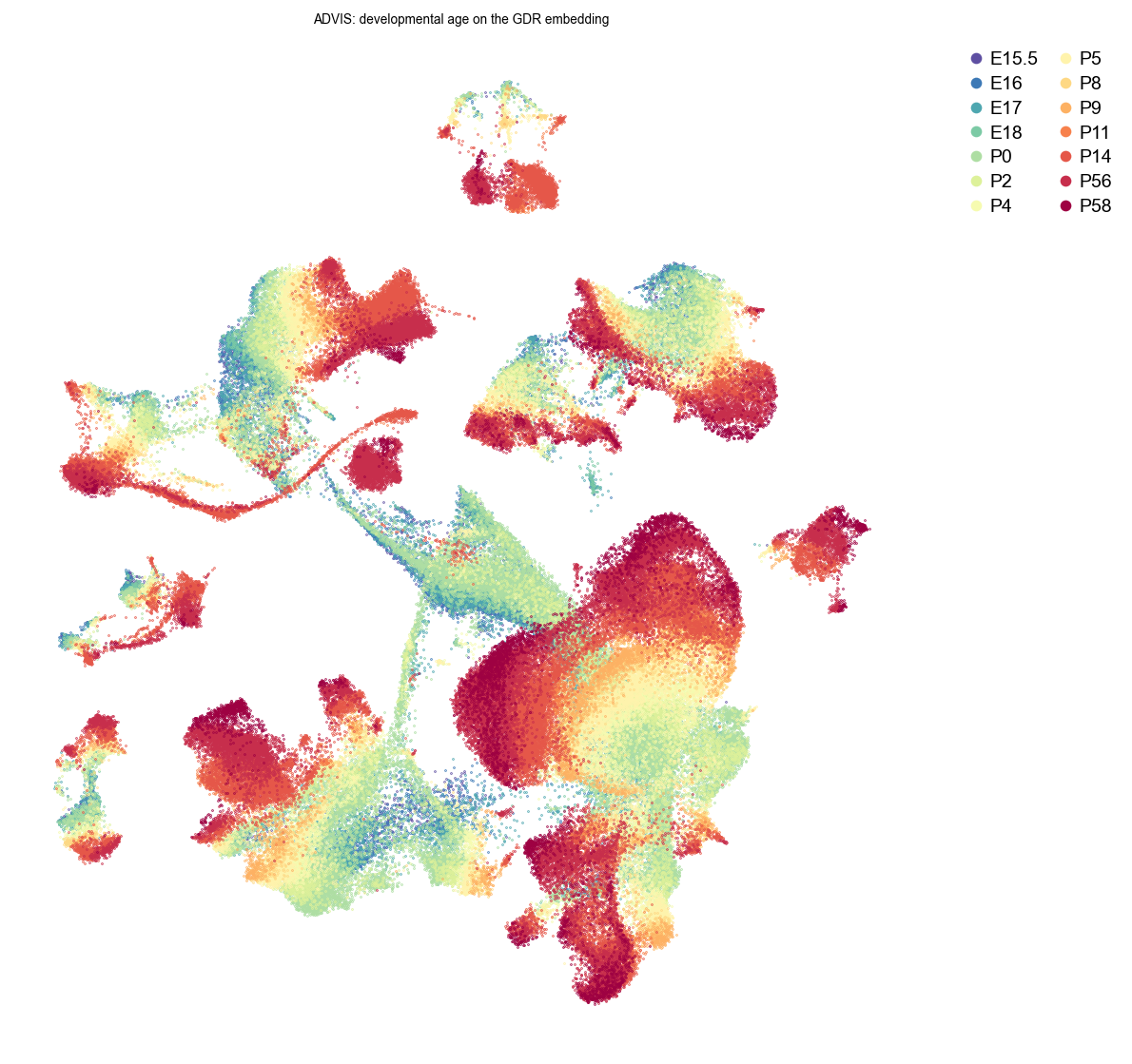
Fourteen ages from E15.5 to P58. The adult timepoints (P56, P58) hold territories of their own, the embryonic and early-postnatal ages grade into each other where the cell types are still differentiating, and the progression is visible without age having been supplied to GDR at any point. Library was removed; age was not — which is the distinction a batch correction has to get right, and the one a single batch-coloured panel cannot show you.

Set the category order explicitly. Sorted as strings, P5 lands after P14 and the legend reads as noise. Any label missing from the order you pass is dropped with a warning, so build the list from the column rather than typing it.

What it costs

step	time	peak RSS
INFOG normalisation	3 m 47 s	1.37 GB
SVD (50 components)	3 m 43 s	1.40 GB
runGDR — stage 1, per-batch INFOG → SVD → neighbours → Leiden	2 m 09 s
runGDR — stage 2, per-batch markers (COSG)	22 s
runGDR — stage 3, scoring every cell against 910 marker sets	1 m 17 s
neighbours + UMAP	5 m 34 s
total	16 m 55 s	5.67 GB

The peak is reached during UMAP, not during GDR: GDR itself peaks at 5.39 GB. For comparison, holding this matrix dense in memory would be 200,061 × 32,285 × 4 bytes ≈ 26 GB before any analysis starts.

The three knobs that trade memory for time

All three are optional. The defaults are sized for a workstation; the reason to touch them is a machine with much more or much less memory than one.

`max_workers` — how many batches are processed at once

Stage 1 spends this budget on outer concurrency, one worker per batch, because each batch’s INFOG and SVD are serial inside. Measured on this dataset:

workers	stage 1	peak RSS
1	244 s	4.2 GB
2	141 s
4	93 s
8	77 s	5.6 GB
20	87 s	9.2 GB

It saturates at eight. Twenty is slower and uses 3.6 GB more, because each worker holds a batch. Eight is the default.

`max_score_batch_cache_bytes` — hold a batch between the two scoring passes

Stage 3 reads each batch twice: once to compute per-feature statistics, once to score. When a batch fits this budget the second read is served from memory instead of being decompressed again — worth about 45% of the first pass.

A batch needs roughly n_cells × nnz_per_cell × 8 bytes. Here the batches run 384 to 13,105 cells, so 11 MB to 370 MB; the 512 MB default (shared by the two concurrent scoring workers) covers 30 of the 35. Raising it to 1 GB covers all of them for about 360 MB more peak. Roughly, it buys 10 seconds per 100 MB until every batch fits, and nothing after that. Set it to 0 to stream twice and use no extra memory.

piaso.tl.runGDR(path, batch_key="library_prep", groupby=None,
                max_score_batch_cache_bytes=1024 * 1024**2)   # all batches cached

`max_score_chunk_bytes` — rows per scoring call

Rows are handed to the scoring kernel in chunks sized from this budget, the dataset’s nonzeros per cell, and the number of marker sets. Past a few thousand rows per call the speed curve is flat, so there is rarely a reason to raise it.

One caveat worth knowing: this value also blocks the first pass’s per-feature sums, so changing it perturbs the embedding in the last bits (order 1e-2 on a score of order 1). It is not a free tuning knob — pin it if you need to reproduce an earlier run exactly.

Reproducibility

runGDR records what it did:

import cytome
ds = cytome.open(path)
print(ds.metadata["X_gdr_params"])       # every parameter, plus the PIASO version
print(ds.metadata["runGDR_marker_genes"])  # the markers each batch contributed
ds.close()

Re-running with the same parameters on the same file gives bit-identical embeddings, including across worker counts: the parallel work unit is chosen for speed and never affects the arithmetic.

If your dataset is bigger

The streaming path has been run at 4.1 million cells: runGDR there took 77 minutes at 1.0 GB of RSS. Memory is a function of the chunk size and the worker count, so a larger dataset costs more time, not more memory.