
Marker-based cell type prediction
predictCellTypeByMarker takes a {cell type: [genes]} dictionary and labels
cells by scoring each set. Three choices decide how well it works, and this
page measures each rather than asserting it: which embedding the scores are
smoothed in, how specific the marker genes are, and where the markers
come from.
import numpy as npimport pandas as pdimport piaso, cosgfrom sklearn.metrics import accuracy_score, silhouette_score
piaso.settings.set_figure_params(style="cell")
1. A reference with labels, and with batches
ref = piaso.data.load_dataset("adult_cortex_multiome_rna")ref.shape, ref.obs["CellTypes"].nunique(), dict(ref.obs["Sample"].value_counts())((17412, 26205), 20, {'1c_TST_NP40_004': 5071, '1c_UC': 4920, '1c_TST': 4364, '1c_without_permiabilization': 2139, '1c': 918})Five preparation protocols, from 918 to 5,071 cells. Worth knowing before embedding anything.
piaso.tl.infog(ref, layer="raw", n_top_genes=3000)layer="raw" is not optional. This dataset keeps counts in a layer and the
integrated matrix in .X; check piaso.data.dataset_info(...)["counts_layer"]
before normalizing anything from the registry. Getting it wrong here does
raise — INFOG checks for integer counts and refuses non-integer input, naming
the layer to pass instead. That guard is why this is a one-line correction
rather than a plausible-looking result you would have to catch later.
2. The embedding
piaso.tl.runSVD(ref, layer="infog", n_components=50, key_added="X_svd")
piaso.tl.runGDR(ref, batch_key="Sample", groupby=None,                layer="infog",                infog_layer="raw",      # per-batch INFOG needs the counts                score_layer="infog",                n_gene=30, key_added="X_gdr", save_reference=True)
batch_key="Sample" makes marker selection run within each protocol, so a
gene that only looks specific because of one protocol’s chemistry cannot become
an axis. groupby=None lets GDR find its own groups per batch.
Note infog_layer="raw" again — GDR re-runs INFOG inside each batch, and
pointing it at .X here produces NaN and a failed SVD. Same trap, second
place.
Measure both embeddings on both questions:
| silhouette, Sample (lower better) | silhouette, CellTypes (higher better) | |
|---|---|---|
| SVD | −0.185 | 0.199 |
| GDR | −0.019 | 0.344 |
Neither embedding separates the protocols: both Sample silhouettes are negative, so there is no batch effect to correct here. What GDR buys is cell type structure: 0.344 against 0.199, a 1.7× improvement on the same cells. That is the argument for it on this dataset, and it is a different argument from batch correction.
piaso.tl.neighbors(ref, use_rep="X_gdr", n_neighbors=15)piaso.tl.umap(ref, use_rep="X_gdr")piaso.pl.embedding(ref, basis="X_umap", color=["Sample", "CellTypes"])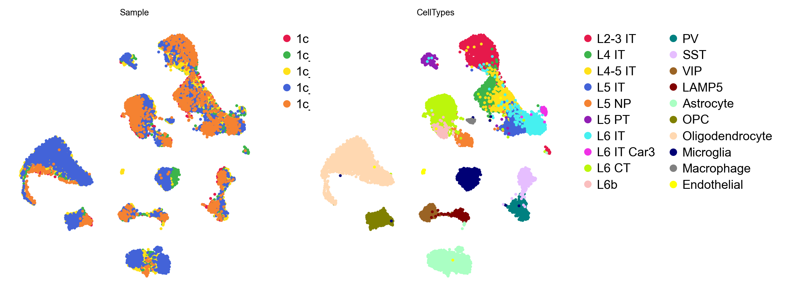
piaso.pl.stackedBarplot(ref, groupby="CellTypes", splitby="Sample")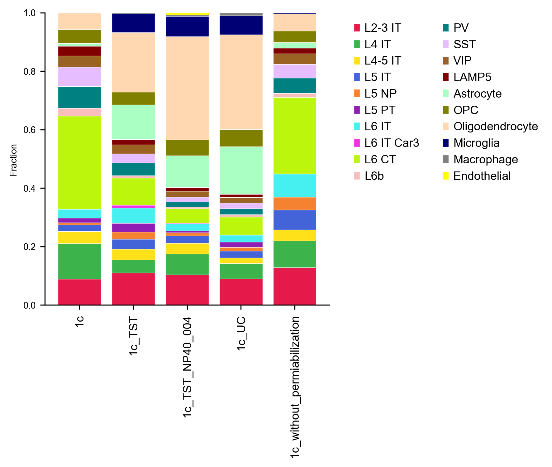
The stacked bars are the check the UMAP cannot give you: if one cell type came overwhelmingly from one protocol, its markers would be protocol markers.
3. Marker genes, and how specific to make them
COSG’s mu penalises genes that are expressed outside the target group. The
default is permissive; raising it trades sensitivity for specificity.
for mu in (1, 10, 100): cosg.cosg(ref, key_added=f"cosg_mu{mu}", groupby="CellTypes", n_genes_user=30 if mu > 1 else 50, mu=mu)Top-30 overlap between mu=1 and mu=10 is 0.87 — about one gene in eight
changes. The ones that change are the point:
| cell type | mu=1 | mu=10 |
|---|---|---|
| PV | 6330411D24Rik, Cemip, Pvalb, Kcnc1, Btbd11, Gpr176 | 6330411D24Rik, Pvalb, Tac1, Cemip, Adamts15, Syt2 |
| Astrocyte | Atp1a2, Plpp3, Gja1, Ntsr2, Sparcl1, Prex2 | Ntsr2, Gja1, Atp1a2, Cldn10, Prex2, Slc39a12 |
At mu=10, PV gains Tac1 and Syt2 — both genuine parvalbumin-interneuron
genes — and Pvalb itself moves up. Astrocytes gain Cldn10. The permissive
setting was spending slots on genes that are merely higher in the group
rather than restricted to it.
30 genes at mu=10 is the setting used below.
names = pd.DataFrame(ref.uns["cosg_mu10"]["names"])marker_sets = {c: list(names[c]) for c in names.columns}4. Predict, and check against held-out truth
rng = np.random.default_rng(0)query = ref[rng.random(ref.n_obs) >= 0.5].copy()
piaso.tl.predictCellTypeByMarker(query, marker_gene_set=marker_sets,                                 score_layer="infog", use_rep="X_gdr",                                 key_added="predicted")
accuracy_score(query.obs["CellTypes"].astype(str), query.obs["predicted"].astype(str))0.95495.4% across 8,738 held-out cells and 20 types. For comparison, the same
data with an SVD embedding and 50 markers at mu=1 gives 0.915 — the
embedding and the marker specificity are worth about four points together.
per_type = (pd.DataFrame({"t": query.obs["CellTypes"].astype(str), "p": query.obs["predicted"].astype(str)}) .groupby("t").apply(lambda d: (d.t == d.p).mean()).sort_values())| worst | best | ||
|---|---|---|---|
| L4-5 IT | 0.578 | Macrophage | 1.000 |
| L6b | 0.779 | Astrocyte | 0.997 |
| L6 IT | 0.812 | OPC | 0.995 |
| L2-3 IT | 0.943 | Microglia | 0.992 |
| L5 IT | 0.945 | VIP | 0.991 |
The pattern from before survives — every remaining error is an excitatory
neuron confused with an adjacent cortical layer, and every glial, vascular and
inhibitory type is near-perfect — but it is much weaker. L6b went from 0.30 to
0.78. L4-5 IT is the residue: a type defined as the boundary between two
others is the hardest thing to call, and no embedding fixes that.
piaso.pl.plotConfusionMatrix(query, groupby_query="predicted", groupby_reference="CellTypes")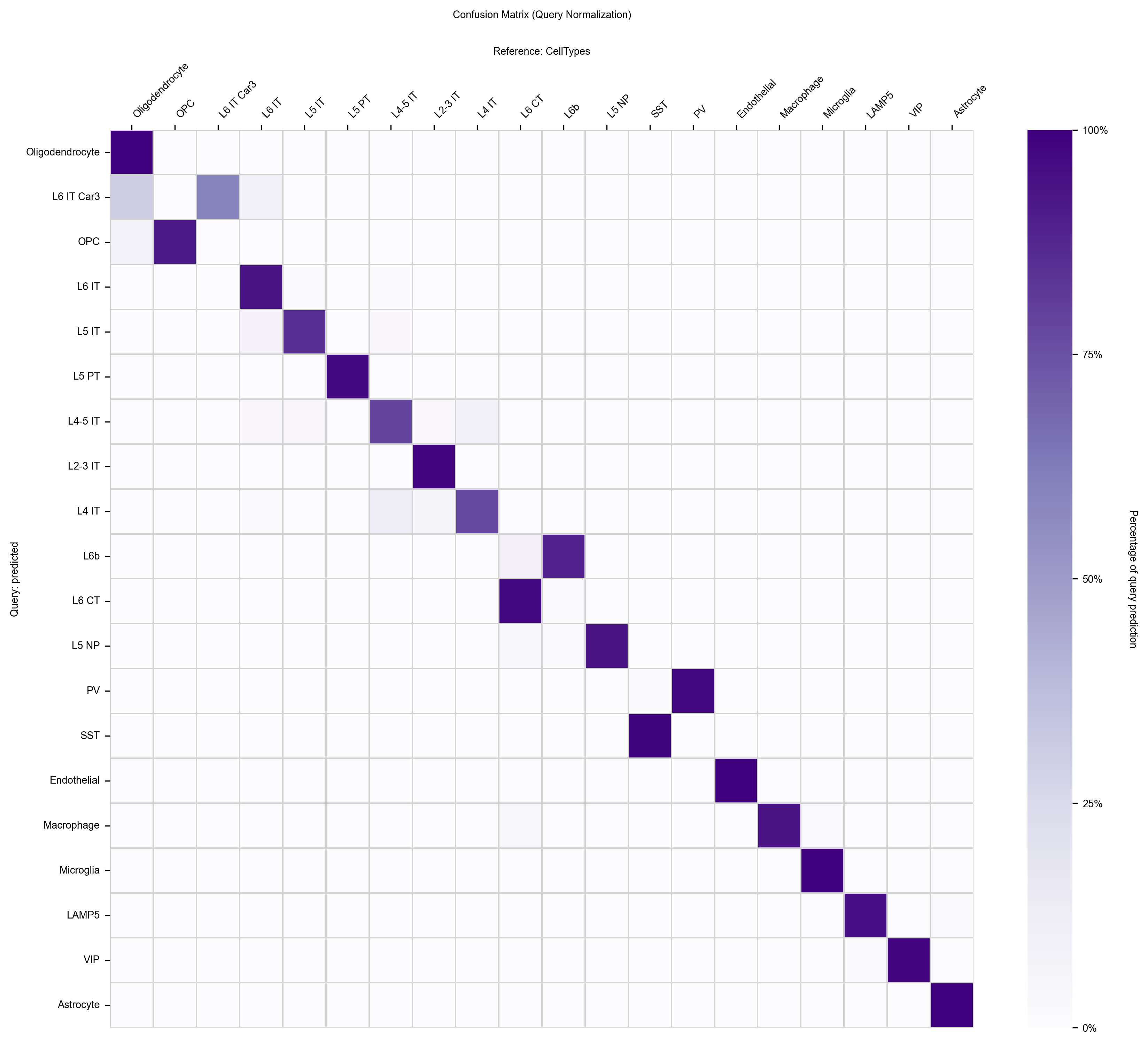
Square cells, one row per predicted label and one column per true label. On this 30% held-out query the two agree for 94.3% of 5,351 cells; what is worth reading is the off-diagonal, which is concentrated between neighbouring cortical layers rather than scattered.
The confusion matrix says it in one look: everything is on the diagonal except a block among the IT layers.
# `predicted` is written as a plain object column, so it carries no category# order and falls back to a sort -- alphabetical against the reference's# biological order, which makes agreement read as a fan rather than a band.# right_order puts both axes in the same order.piaso.pl.sankey(query, left="CellTypes", right="predicted", right_order=query.obs["CellTypes"].cat.categories)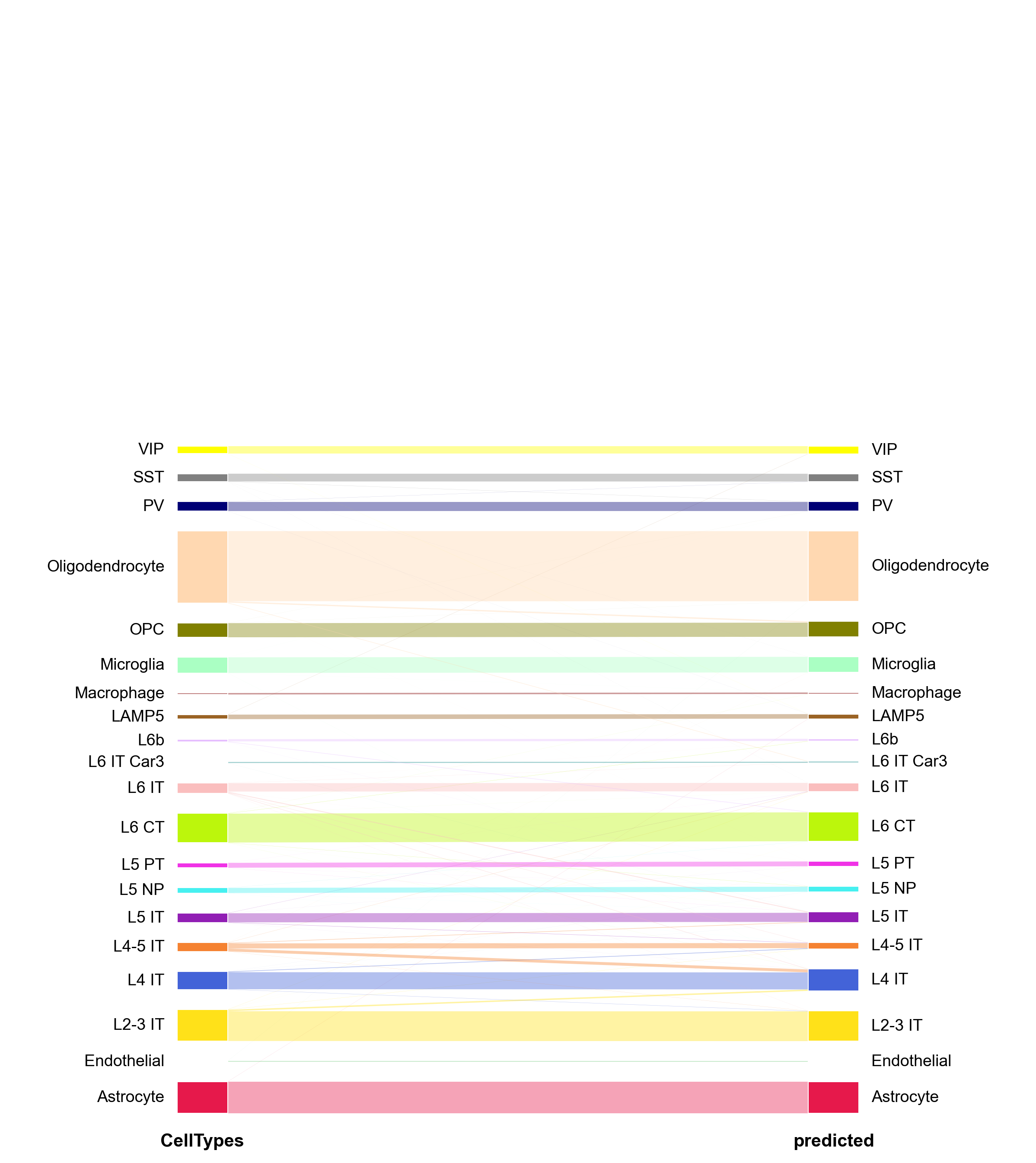
A Sankey answers a different question from a confusion matrix: it shows where the cells went, weighted by how many there are, so a 58% accurate type with few cells does not dominate the picture.
metrics = pd.DataFrame({"accuracy": per_type, "n_cells": query.obs["CellTypes"].value_counts()}).dropna()piaso.pl.plotGroupMetrics(metrics)
Plotting accuracy against group size together is the honest summary: it shows at a glance that the poor calls are not the rare types.
5. The same call against PIASOmarkerDB
Nothing changes except where the dictionary comes from:
db = piaso.tl.getMarkers(study="AllenWholeMouseBrain_isocortex",                         as_dict=True)covered = {k: [g for g in v if g in query.var_names] for k, v in db.items()}covered = {k: v for k, v in covered.items() if len(v) >= 5}
piaso.tl.predictCellTypeByMarker(query, marker_gene_set=covered,                                 score_layer="infog", use_rep="X_gdr",                                 key_added="predicted_db")
The database uses the Allen whole-mouse-brain taxonomy, whose names share nothing with this reference’s. Cross-tabulating asks whether two independently annotated datasets agree about the same cells:
| reference label | PIASOmarkerDB label | cells |
|---|---|---|
| Oligodendrocyte | 327 Oligo NN | 2,132 |
| Astrocyte | 319 Astro-TE NN | 959 |
| L6 CT | 030 L6 CT CTX Glut | 887 |
| L2-3 IT | 007 L2/3 IT CTX Glut | 801 |
| Microglia | 334 Microglia NN | 476 |
| OPC | 326 OPC NN | 433 |
| PV | 052 Pvalb Gaba | 278 |
Every row is the correct correspondence. That is the check worth doing before trusting an annotation: not “does the UMAP look right”, but “do two independent sources agree about these cells”.
On the embedding, the database’s vocabulary lands on the same territories as the reference’s:
piaso.pl.embedding(query, basis="X_umap", color=["CellTypes", "predicted_db"], ncol=1)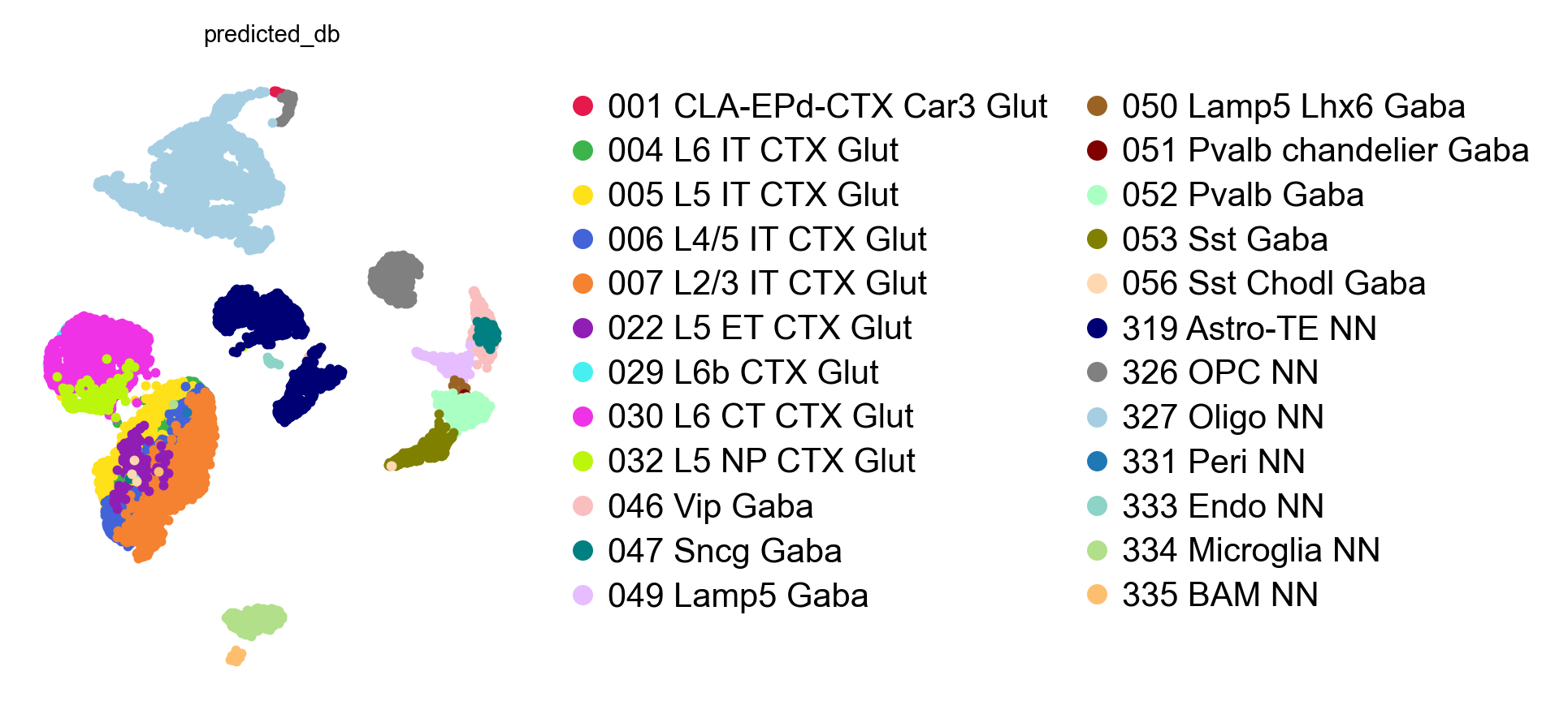
The two panels use names that share nothing — Oligodendrocyte against
327 Oligo NN — and draw the same map. That is the useful reading of a Sankey
or a cross-tabulation put back on the cells: agreement between sources that
could not have copied each other.
Which source to use
- Your own reference, when you have one from the same tissue and protocol: better matched, and the vocabulary your collaborators use.
- PIASOmarkerDB, when you do not: 36 studies across human and mouse. See the API client page, which also covers annotating clusters rather than cells.
- Match the developmental stage. An adult taxonomy asked to label embryonic tissue gives confident, wrong answers: worked through in cells vs nuclei.
Parameters worth knowing
| parameter | what it changes |
|---|---|
use_rep | the embedding smoothing runs in. X_gdr beat X_svd by ~4 points here. |
score_layer | which matrix the marker sets are scored on. Defaults to infog. |
smooth_prediction | average each cell’s scores over its neighbours. On by default; needs use_rep. |
COSG’s mu | specificity penalty on the markers. 10 was better than 1 here. |
Related
- projectGDR — reuse this reference’s GDR space for a new dataset, without recomputing it.