GDR beyond cell types

GDR builds an embedding from the genes that distinguish labelled groups. Nothing in that idea is specific to genes, or to cell types. This page runs it on two datasets that are not a tissue — handwritten digits, clothing photographs, and a differentiation trajectory — because what a method does on data it was not designed for is the clearest statement of what it actually does.

The result is consistent and it cuts both ways. On all three, GDR separates the known groups substantially better than an SVD embedding, and predicts labels from neighbours slightly worse. Both halves are worth knowing before reaching for it.

import numpy as np
import pandas as pd
import anndata as ad
import piaso, cosg
from sklearn.metrics import silhouette_score
from sklearn.neighbors import KNeighborsClassifier
from sklearn.model_selection import train_test_split

1. Fashion-MNIST as an expression matrix

A 28×28 greyscale image is a 784-dimensional vector. Call each pixel a gene and each image a cell, and the whole pipeline runs unchanged:

from sklearn.datasets import fetch_openml
fm = fetch_openml("Fashion-MNIST", version=1, as_frame=False, parser="liac-arff")

rng = np.random.default_rng(0)
idx = rng.choice(fm.data.shape[0], 20000, replace=False)
LABELS = ["T-shirt/top", "Trouser", "Pullover", "Dress", "Coat",
          "Sandal", "Shirt", "Sneaker", "Bag", "Ankle boot"]

a = ad.AnnData(np.asarray(fm.data[idx], dtype="float32"))
a.var_names = [f"px{i}" for i in range(a.n_vars)]
a.obs["label"] = pd.Categorical([LABELS[int(v)] for v in fm.target[idx]])
a.layers["raw"] = a.X.copy()

fetch_openml reaches Fashion-MNIST and MNIST directly — torchvision is not needed, which is worth saying because the obvious assumption is that it is.

piaso.tl.infog(a, layer="raw", n_top_genes=400)
piaso.tl.runSVD(a, layer="infog", n_components=50, key_added="X_svd")
piaso.tl.neighbors(a, use_rep="X_svd", n_neighbors=15)
piaso.tl.umap(a, use_rep="X_svd")
piaso.pl.embedding(a, basis="X_umap", color="label")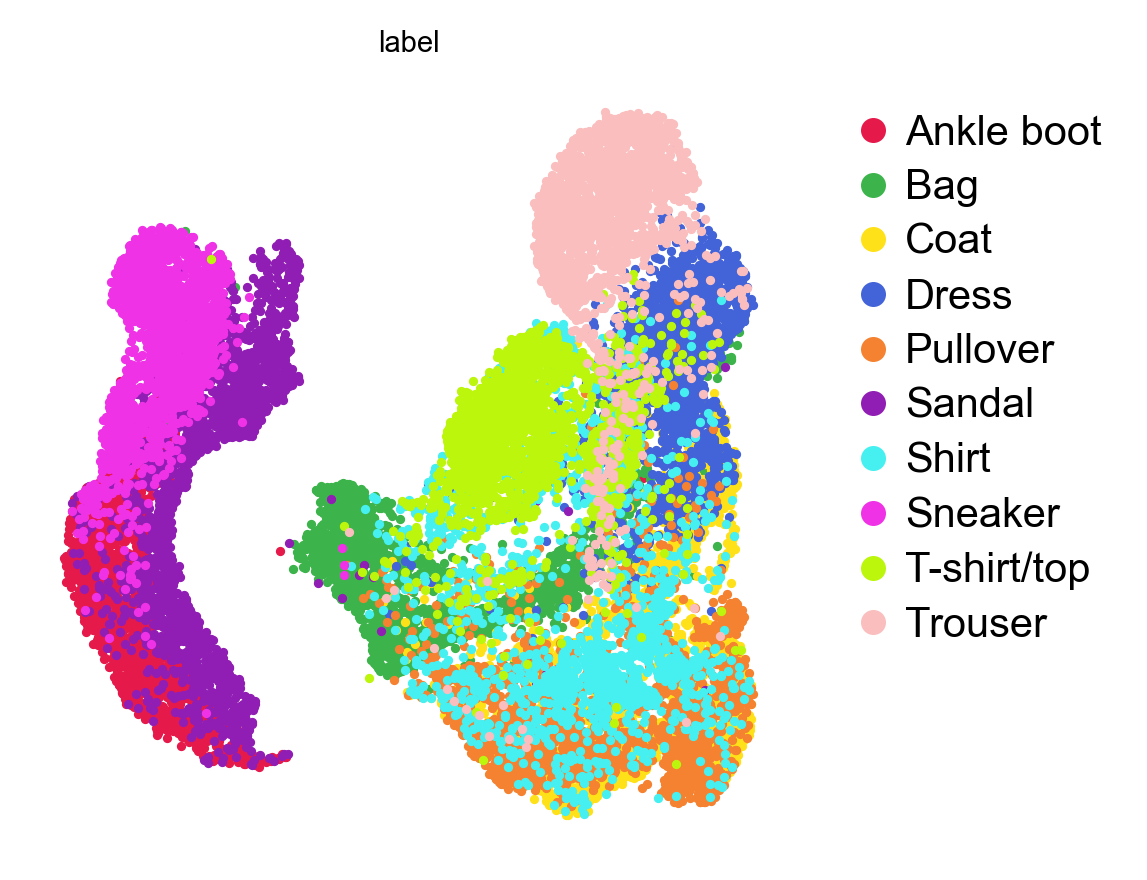

piaso.tl.runGDR(a, batch_key=None, groupby="label", n_gene=30, mu=10,
                layer="infog", score_layer="infog")
piaso.tl.neighbors(a, use_rep="X_gdr", n_neighbors=15)
piaso.tl.umap(a, use_rep="X_gdr", key_added="X_umap_gdr")
piaso.pl.embedding(a, basis="X_umap_gdr", color="label")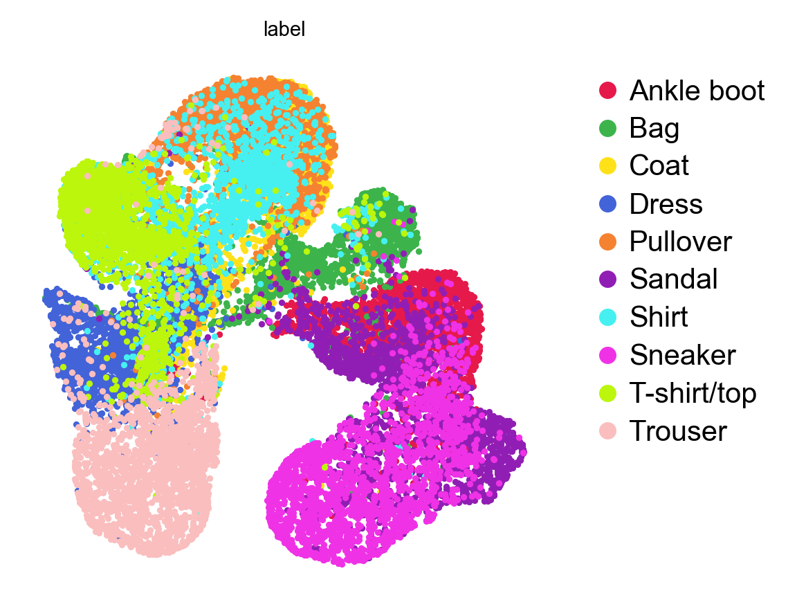

2. Which pixels are “marker genes”

COSG on pixels asks which pixels are specific to a garment class, and the answer can be looked at directly — the one thing you cannot do with real genes:

cosg.cosg(a, groupby="label", key_added="cosg", n_genes_user=30, mu=10,
          layer="infog")
names = pd.DataFrame(a.uns["cosg"]["names"])
selected = sorted({int(g[2:]) for c in names.columns for g in names[c]})
len(selected)

268     # of 784 pixels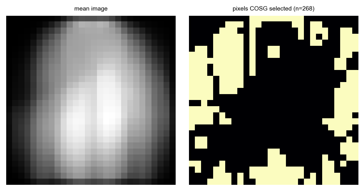

Mean image, and the pixels COSG selected

268 pixels of 784, and they are not scattered: they concentrate where garment silhouettes differ — the shoulder line, the gap between trouser legs, the sole of a shoe. The dark border, where every image is empty, contributes nothing and is dropped. That is the same behaviour as on a transcriptome, where housekeeping genes are uninformative because they are the same everywhere.

3. Pancreatic endocrinogenesis: a trajectory, not clusters

Cell types are discrete. A differentiation trajectory is not, and it is the harder case for a method that builds its space from group-specific features.

p = ad.read_h5ad("endocrinogenesis_day15.h5ad")   # ~52 MB, direct download
p.layers["raw"] = p.X.copy()
p.obs["clusters"].value_counts()

Ductal           916
Ngn3 high EP     642
Pre-endocrine    592
Beta             591
Alpha            481
Ngn3 low EP      262
Epsilon          142
Delta             70

Ductal → Ngn3-low → Ngn3-high → pre-endocrine → the four hormone-producing fates. Neighbouring stages are genuinely continuous with each other.

piaso.tl.infog(p, layer="raw", n_top_genes=3000)
piaso.tl.runSVD(p, layer="infog", n_components=50, key_added="X_svd")
piaso.tl.neighbors(p, use_rep="X_svd", n_neighbors=15)
piaso.tl.umap(p, use_rep="X_svd")
piaso.pl.embedding(p, basis="X_umap", color="clusters")

piaso.tl.runGDR(p, batch_key=None, groupby="clusters", n_gene=30, mu=10,
                layer="infog", score_layer="infog")
piaso.tl.neighbors(p, use_rep="X_gdr", n_neighbors=15)
piaso.tl.umap(p, use_rep="X_gdr", key_added="X_umap_gdr")
piaso.pl.embedding(p, basis="X_umap_gdr", color="clusters")

4. The trade, in two numbers

Separation of the known groups (silhouette) against the ability to predict a label from neighbours (15-NN accuracy, 70/30 split):

dataset	silhouette SVD → GDR	15-NN accuracy SVD → GDR
MNIST digits	0.05 → 0.15	0.912 → 0.788
Fashion-MNIST	0.038 → 0.104	0.817 → 0.767
Pancreas (8 stages)	0.100 → 0.309	0.886 → 0.870

def knn_acc(X, y, seed=0):
    Xtr, Xte, ytr, yte = train_test_split(X, y, test_size=0.3,
                                          random_state=seed, stratify=y)
    return KNeighborsClassifier(15).fit(Xtr, ytr).score(Xte, yte)

y = p.obs["clusters"].astype(str).values
for key in ("X_svd", "X_gdr"):
    print(key, knn_acc(p.obsm[key], y),
          silhouette_score(p.obsm[key], y, sample_size=3000, random_state=0))

Silhouette improves every time — by 3× on the pancreas — and kNN accuracy drops every time. These are not in tension; they measure different things.

GDR builds its axes from the genes that separate the labelled groups, so the groups end up compact and far apart: that is the silhouette. Getting there means discarding everything those genes do not capture, including the local variation kNN was using to interpolate between neighbours. On the pancreas the cost is small (0.886 → 0.870) because the discarded variation was mostly noise. On MNIST it is large (0.912 → 0.788) because 30 pixels per digit class throw away real, usable signal — a digit is defined by its whole shape, not by 30 diagnostic points.

So the honest rule is: GDR is a structure method, not a classifier. Use it when you want the biology organised by what distinguishes your groups — for comparing across samples, projecting onto a reference, or seeing sub-structure that variance-driven axes bury. If the goal is to predict labels for new observations, an embedding that retains more of the data will usually do better.

The pancreas is the case that makes the point cleanly: a 3× better-separated trajectory for a 1.6% accuracy cost. That is a good trade, and it is a trade, which is why both numbers are here.

Notes

n_gene=30 per group is the parameter that sets how aggressive the compression is. Raising it recovers kNN accuracy and lowers separation.
The images use n_top_genes=400 (of 784 pixels) rather than 3,000: INFOG cannot select more features than exist.
Fashion-MNIST is subsampled to 20,000 of 70,000 images purely for runtime; the full set behaves the same.

GDR — the method, on the data it was built for.
projectGDR — freezing a GDR space and projecting new data into it, which is where the structure-vs-classifier distinction matters most.