
Xenium into a cytome directly, without building an AnnData
The Xenium tutorial builds an AnnData, clusters it, and converts the result to a cytome. That is the right route when you already have an AnnData workflow, or when the analysis you want lives in scanpy.
This is the other route: the matrix goes from 10x files straight into a cytome, and every step after that reads from the file. Same data, same figure at the end, no in-memory object holding the matrix at any point.
Which to use is a workflow question, not a correctness one:
| AnnData first | cytome-native (this page) | |
|---|---|---|
| entry | sc.read_10x_h5 → AnnData → from_anndata | cytome.from_10x_h5 |
| matrix in memory | yes, whole | never |
| scanpy interop | immediate | via to_anndata when you want it |
| best when | the analysis is scanpy-shaped, or the section is small | the section is large, or it is one of many |
1. The matrix, in one call
Xenium’s cell_feature_matrix.h5 is a 10x-format matrix, so it needs no
intermediate object:
import cytome
ds = cytome.from_10x_h5("cell_feature_matrix.h5", output="xenium.cytome")ds.n_cells, ds.n_genes        # 167780, 313
UserWarning: 228 features of type ['Blank Codeword', 'Negative ControlCodeword', 'Negative Control Probe'] were not written: only 'Gene Expression'(-> RNA) and 'Peaks' (-> ATAC) map to a cytome modality.Read that warning rather than silencing it: Xenium panels ship negative controls and blank codewords alongside the 313 real probes, and they are not expression. They are worth keeping for QC — read them from the h5 directly — but they do not belong in the RNA modality, and the importer says so instead of quietly averaging them into your data.
11 seconds for 167,780 cells.
2. Coordinates, and the index that comes with them
cells.csv.gz carries the centroids. Align it to the cytome’s own barcode
order rather than assuming the two files agree:
import pandas as pd, numpy as np
cells = pd.read_csv("cells.csv.gz")cells["cell_id"] = cells["cell_id"].astype(str)          # ints vs stringsbc = np.asarray(ds.cells["barcode"]).astype(str)cells = cells.set_index("cell_id").reindex(bc)           # reindex, don't zipassert not cells[["x_centroid", "y_centroid"]].isna().any().any()
xy = cells[["x_centroid", "y_centroid"]].to_numpy(dtype=np.float32)ds.add_embedding("spatial", xy)ds.set_spatial_coords(xy)        # builds the R*-tree for cells_in_regionds.flush()
reindex on the barcode is the step that matters. The two files are in the
same order today; a filtered matrix or a re-exported csv breaks that silently,
and a positional zip would attach every coordinate to the wrong cell without
raising.
3. Normalise, embed and cluster — all from the file
import piaso
piaso.tl.infog(ds, modality="RNA", layer="counts", key_added="infog", save_layer=True, inplace=True)piaso.tl.runSVD(ds, layer="infog", n_components=30, key_added="X_svd")piaso.tl.neighbors(ds, use_rep="X_svd", n_neighbors=15)piaso.tl.leiden(ds, resolution=0.3, key_added="leiden")ds.flush()| step | time |
|---|---|
from_10x_h5 | 11 s |
| INFOG | 11 s |
| SVD (30 components) | 10 s |
| neighbours + Leiden | 25 s |
Under a minute end to end on 167,780 cells, and nothing above returns a matrix.
4. The image, and the overlay
ds.add_spatial_image("xenium", "morphology", "morphology_mip.ome.tif")ds.flush()
piaso.pl.plotEmbedding(ds, color="leiden", basis="spatial", image=True,                       img_key="morphology", image_alpha=0.7, legend_loc=None)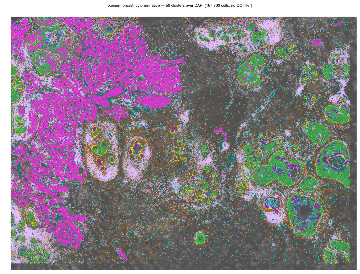
The ducts read as rings of one cluster against the stroma, which is the same structure the AnnData route finds — the point being that it is the same structure, reached without the matrix ever being in memory.
5. One difference worth explaining
This page gets 58 clusters where the AnnData page gets 29, and the cause is not the backend. The AnnData route filters cells first; this one does not, so 167,780 cells go into the clustering against 164,000, and the extra ones are mostly low-count cells that fragment into small clusters.
Filter on the cytome if you want the two to match:
counts = np.asarray(ds.cells["transcript_counts"])keep = np.where(counts >= 10)[0]piaso.pl.plotEmbedding(ds, color="leiden", basis="spatial", cell_mask=keep)cell_mask plots the subset without writing a second file. To make the
filter permanent, cytome.filter_cells writes a new cytome — and note that
a filtered file needs its GTF re-imported if it had one.
Where to go next
- Regions of interest
—
cells_in_regionandspatial_images.cropwork identically here, becauseset_spatial_coordsabove built the same index. - Regulons on a spatial section — the same file shape, one analysis further on.