
cytorete on spatial data: regulons across a whole embryo
cytorete infers regulons from RNA:
promoter motifs crossed with trans co-specificity across cell types. That
recipe never mentions dissociation, so it works unchanged on spatial
transcriptomics — and spatial data makes the result legible, because a
regulon’s activity can be drawn where the tissue actually is.
This runs the whole thing on one Stereo-seq section: an E16.5 mouse
embryo, 121,767 bins, 25 annotated organs, streamed from a .cytome.
The dataset ships with the authors’ own SCENIC regulons, which makes it a rare thing in a tutorial — an independent method to check against on the same tissue. Section 4 does exactly that.
1. The section
Start from the rotated embryo produced in the
Stereo-seq spatial tutorial — same file, already
carrying annotation and an upright spatial embedding.
import piasoimport cytome, piaso, cytorete
ds = cytome.open("mosta_rot.cytome")ds.n_cells          # 121767piaso.settings.set_figure_params(style="cell")   # one house style across every figure
INFOG needs raw counts, and this dataset keeps them in a layer rather than
in X:
piaso.tl.infog(ds, modality="RNA", layer="count", key_added="infog", save_layer=True, inplace=True)ds.flush(); ds.close()MOSTA does ship raw counts —
layers['count'], int64, in this section ranging 1–219. What it does not do is put them inX, which holds log-normalized values. Passing those would make INFOG return numbers that look fine and mean nothing, so PIASO checks for integers and refuses, naming the layer to use instead.Mind the name: the raw layer is
count, singular. After conversion the cytome also hascounts— the normalized matrix that came fromX. One letter apart, and only one of them is countable.
2. One call, 121,767 bins
TFS = ["Sox2", "Pax6", "Sox10", "Foxa2", "Hnf4a", "Myod1", "Myog",       "Gata4", "Twist1", "Grhl3", "Cdx2", "Olig1", "Lhx2", "Emx2", "Tbx5"]
cytorete.inferRegulon(    "mosta_rot.cytome", "mm10", "annotation",    jaspar_path=piaso.data.fetch_jaspar(),    twobit_path=piaso.data.fetch_2bit("mm10"),    tf_list=TFS, cosg_layer="infog", score_layer="infog")
inferRegulon takes the path directly and closes the file when it is done.
tf_list is what bounds the run — the log’s 14 TFs is 14 of the 15
requested, not a ceiling the data imposed. Omit tf_list to use every
expressed TF that has a motif.
From the run log:
[inferRegulon] 14 TFs with motifs in the data[inferRegulon] target_genes='cosg' → 3464 genes to scan[inferRegulon] 3301 genes with promoters (5350 intervals)[cistrome] M = 14 TFs × 3301 genes, 3602 edges (7.79% density)cospecificity_trans: 920 positive-sign edges over 25 cell types[regulons] 11 global regulons (median 72 targets); per-cell-type for 19[regulonActivity] scoring 11 regulons (layer=infog, pvalues=True)29 s for the regulon step on 121,767 bins × 28,204 genes, ~1 GB of RSS, because the matrix is streamed and never held whole.
Four of the fifteen TFs drop out, at two different stages, and the log distinguishes them:
-
Grhl3has no motif in JASPAR2024 CORE vertebrates — it is the only one of the fifteen that is missing, which is why the line reads 14 TFs. That is a gap in the motif database, not a species mismatch: CORE vertebrates is cross-species and stores names in HGNC form (SOX2,MYOD1), matched case-insensitively, so mouse symbols resolve fine. -
Sox10,Lhx2andEmx2have motifs but lose their regulons: each came out of the co-specificity step with zero surviving targets, well undermin_targets(default 10). Not marginal — nothing at all.The reason is the annotation, not the TF. All three are restricted within a single label here:
Sox10to glia and neural crest,Lhx2andEmx2to cortical progenitors — and this section is annotated at organ level, so all three live insideBrain. Co-specificity asks whether a TF and a candidate target vary together across the grouping; a TF confined to one group has nothing to vary against, and scores zero by construction. Sub-annotate the brain and they return. A TF dropping out this way is a statement about the resolution of your labels.
To scan a TF whose motif JASPAR lacks, add CIS-BP (motif_db="both",
cisbp_dir=piaso.data.fetch_cisbp()), which covers many TFs JASPAR does
not.
3. Where a regulon is active
Activity lands in the X_regulon embedding, one column per regulon. Read
the column order from the store, never from your TF list — dropped TFs and
per-cell-type regulons both change it:
import json, numpy as np
ds = cytome.open("mosta_rot.cytome")md = ds.metadata["regulon"]md = json.loads(md) if isinstance(md, str) else mdnames = md["names"]                      # authoritative column orderA = np.asarray(ds.embeddings["X_regulon"])
for tf in names:                          # as columns, to plot by name    ds.cells[f"regulon_{tf}"] = A[:, names.index(tf)]ds.flush()
# activity, and the p-value from the same control-set nullP = np.asarray(ds.embeddings["X_regulon_pval"])for tf in ["Sox2", "Myog", "Hnf4a", "Twist1"]:    ds.cells[f"neglog10p_{tf}"] = -np.log10(np.clip(P[:, names.index(tf)], 1e-300, 1))ds.flush()
for tf in ["Sox2", "Myog", "Hnf4a", "Twist1"]:    piaso.pl.plotEmbedding(ds, color=f"regulon_{tf}",   basis="spatial",                           vmin_pct=10, vmax_pct=90)     # top row    piaso.pl.plotEmbedding(ds, color=f"neglog10p_{tf}", basis="spatial")                                                          # bottom row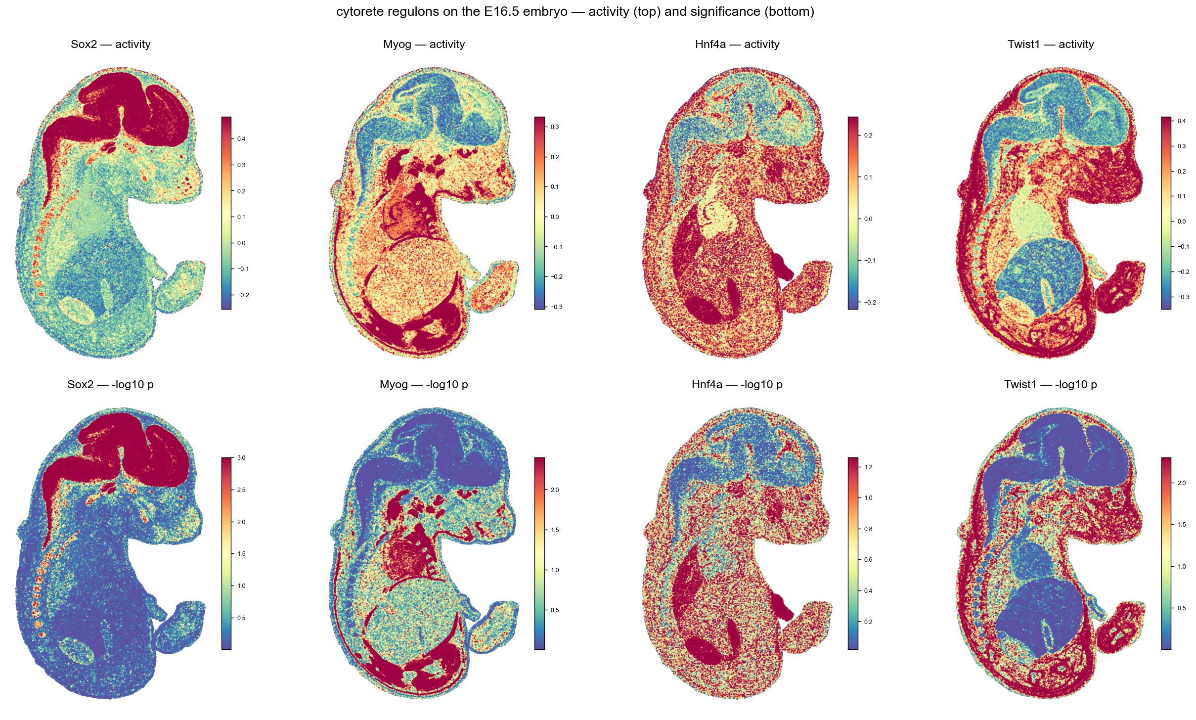
vmin_pct/vmax_pct clip the colour range to percentiles, and only the
activity row needs them: activity is skewed, Spectral_r has a pale
midpoint, and without clipping a handful of extreme bins own the scale.
10/90 is what this data needed — 2/98 was still too narrow.
The p-value row takes no clipping. -log10(p) is already bounded: the
permutation floor caps it at log10(n_ctrl + 1), so the scale is fixed by
the test rather than by outliers, and clipping it would only hide the
ceiling.
The bottom row is -log10(p) against the control-set null. Sox2 is
significant across brain and spinal cord, Myog through the musculature; and
the ceiling is the permutation floor, so a saturated panel means “as
significant as this test can report”, not “infinitely so”.
Nothing in the inference knew where any bin was — annotation labels went
in, coordinates did not. The anatomy is a readout, not an input:
| Regulon | Where it lights up |
|---|---|
| Sox2 | brain and choroid plexus, plus the dorsal root ganglion chain down the back |
| Myog | skeletal muscle — intercostals, tongue, limb muscle |
| Hnf4a | a tight liver and gut focus |
| Twist1 | mesenchyme everywhere except brain and liver |
Ranking organs by mean activity says the same thing in numbers:
Sox2 Brain, Choroid plexus, Inner earMyog Muscle, Heart, Connective tissueHnf4a GI tract, Smooth muscle, KidneyOlig1 Sympathetic nerve, Brain, Dorsal root ganglionTwist1 Adipose tissue, Cartilage primordium, EpidermisCdx2 GI tract, Adrenal gland, Smooth muscle4. Against the published regulons
The MOSTA authors ran SCENIC on this section and shipped the per-bin scores
as obs columns (Regulon - Sox2, …). Two methods, same tissue, no shared
code, so this is a real check rather than a self-comparison.
from scipy.stats import spearmanr
def cosine(a, b):                      # centred, so it is not driven by offset    a, b = a - a.mean(), b - b.mean()    return float(a @ b / (np.linalg.norm(a) * np.linalg.norm(b)))
for tf in names:    j = names.index(tf)    ref = np.asarray(ds.cells[f"Regulon - {tf}"], dtype=float)    ok = np.isfinite(ref) & np.isfinite(A[:, j])    print(tf, round(spearmanr(A[ok, j], ref[ok]).statistic, 3),              round(cosine(A[ok, j], ref[ok]), 3))
Both metrics are reported because they answer different questions: Spearman asks whether the two rank the bins the same way, cosine whether the score shapes line up. They agree here, which is the useful outcome — a disagreement between them would mean the ranking and the magnitudes were telling different stories.
# activity, significance, and the published score, on the same colour rulesfor tf in ["Sox2", "Olig1"]: for col in (f"regulon_{tf}", f"neglog10p_{tf}", f"Regulon - {tf}"): piaso.pl.plotEmbedding(ds, color=col, basis="spatial", vmin_pct=10, vmax_pct=90)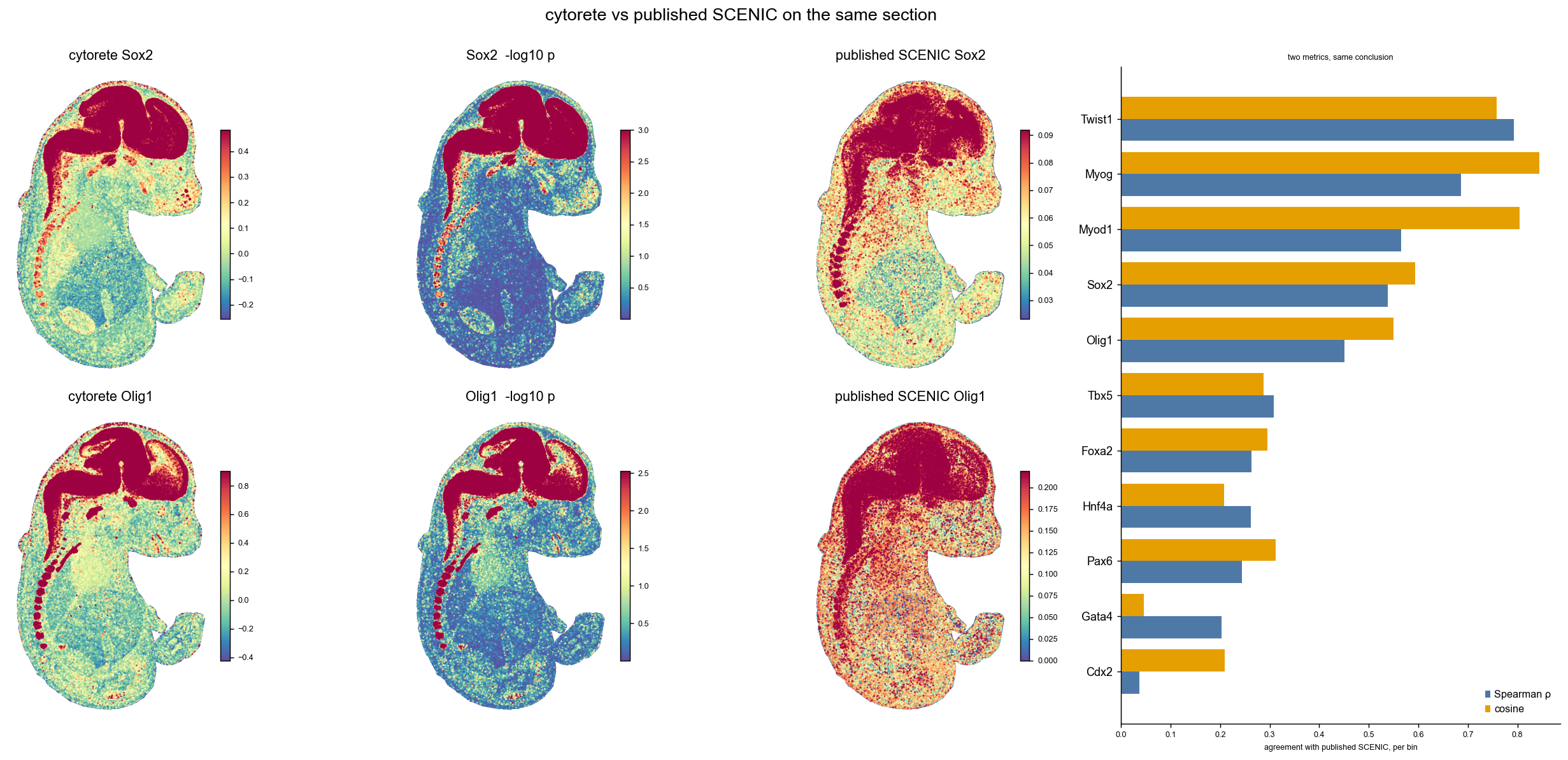
All eleven agree positively, median ρ = +0.31, and cosine tracks it: Twist1 0.79/0.76, Myog 0.69/0.84, Myod1 0.57/0.81, Sox2 0.54/0.59, down to Cdx2 at 0.04/0.21.
Where the two disagree, and which is more plausible
Ranking each method by how much it enriches its regulon in the expected organ (mean inside minus mean outside, in SD units) splits the set cleanly, and not in one direction:
| regulon | expected | cytorete | SCENIC | favours |
|---|---|---|---|---|
| Sox2 | Brain | 2.16 | 1.43 | cytorete |
| Olig1 | Brain | 1.98 | 1.32 | cytorete |
| Myog | Muscle | 2.67 | 3.14 | SCENIC |
| Hnf4a | Liver | 0.12 | 2.75 | SCENIC |
| Gata4 | Heart | −0.41 | 2.56 | SCENIC |
| Cdx2 | GI tract | 2.46 | 4.52 | SCENIC |
The honest summary is that cytorete is sharper on the neural regulons and SCENIC on the endoderm and heart ones — not that either dominates.
The clearest single case is in the figure. SCENIC’s Olig1 is close to uniform across the whole embryo, including limb, liver and gut; cytorete’s is restricted to brain and the dorsal root ganglion chain. Olig1 is a CNS factor — ventral neural tube progenitors and the oligodendrocyte lineage — so a body-wide signal at E16.5 is not a plausible readout, and the restricted one is. Sox2 shows the same pattern more mildly.
The reverse cases are worth taking equally seriously. cytorete’s Gata4 regulon is negatively enriched in heart here, and its top regions come out as GI tract and smooth muscle. Gata4 is genuinely active in both gut and heart, so this is not nonsense, but on this section the published regulon places it better. A method comparison that only reported Sox2 and Olig1 would be selecting its own evidence.
5. Notes for your own section
- Read
md["names"]for the column order. Building it from your input TF list breaks silently the moment a TF drops out for want of a motif. - Check which layer is raw.
countvscountsdiffered by one letter in this dataset and one of them was normalized. tf_listis optional. Omit it to run every expressed TF with a motif; it is slower and the plots get busier, but nothing else changes.- Per-cell-type regulons are in
md["per_celltype"]— the same TF can carry a different target set in brain than in muscle, which is the point of inferring them per cell type rather than once for the section.