
Motif analysis: sequence, PWMs and what a hit is worth
Scanning is the easy half. piaso.data fetches the genome and the motif
databases, piaso.pp.scan_motifs finds the hits, and the Rust backend does it
91× faster than numpy. The half that decides whether the answer means
anything is what you compare against, and this page contains a result that
looks completely convincing and is entirely an artefact.
Everything here is in pip install piaso-tools. Reading sequence from a
.2bit needs one optional package:
# pip install py2bitimport numpy as npimport pandas as pdimport piasofrom scipy.stats import fisher_exactfrom statsmodels.stats.multitest import multipletests
piaso.settings.set_figure_params(style="cell")
1. The genome
piaso.data keeps a small cache of genome files and tells you what it has:
piaso.data.list_available_genomes()['hg38', 'mm10']files = piaso.data.resolve_genome_files("hg38")sorted(files)['chrom_sizes', 'ctcf', 'gene_boundary', 'gtf', 'promoter', 'tss_bed']tss_bed is one row per transcript — 146,857 of them — which is what promoter
windows are built from.
tss = pd.read_csv(files["tss_bed"], sep="\t", header=None, names=["chrom", "start", "end", "gene", "score", "strand", "biotype", "gene_id", "tx_id"])tss.shape(146857, 9)2. Promoter windows
TSS − 1000 to TSS + 500, on the gene’s strand. A minus-strand gene’s upstream is to the right in genome coordinates; getting this backwards silently scans the wrong 1.5 kb and produces a clean-looking wrong answer.
UP, DOWN = 1000, 500
def promoters(genes):    """One window per gene, from its first listed TSS."""    sub = tss[tss["gene"].isin(genes)].drop_duplicates("gene")    rows = []    for r in sub.itertuples():        lo, hi = ((r.start - UP, r.start + DOWN) if r.strand == "+"                  else (r.start - DOWN, r.start + UP))        rows.append((r.gene, r.chrom, max(0, lo), hi, r.strand))    return pd.DataFrame(rows, columns=["gene", "chrom", "start", "end", "strand"])
3. Gene sets: human brain cell classes
Marker sets from an atlas beat a hand-picked list: they are bigger, and they were not chosen by someone who already had a hypothesis about which motifs would win. SEA-AD middle temporal gyrus gives 24 subclasses, 50 markers each:
marker_db = piaso.tl.getMarkers(study="SEAAD2024_MTG_Subclass", as_dict=True)len(marker_db), sorted(marker_db)[:6](24, ['Astrocyte', 'Chandelier', 'Endothelial', 'L2/3 IT', 'L4 IT', 'L5 ET'])Group them into classes, so each class has enough promoters to test:
CLASSES = { "Glia": ["Astrocyte", "Oligodendrocyte", "OPC", "Microglia-PVM"], "Excitatory": ["L2/3 IT", "L4 IT", "L5 IT", "L6 IT", "L5 ET", "L6 CT", "L5/6 NP", "L6b", "L6 IT Car3"], "Inhibitory": ["Pvalb", "Sst", "Vip", "Lamp5", "Sncg", "Chandelier", "Pax6", "Lamp5 Lhx6"], "Vascular": ["Endothelial", "VLMC"],}sets = {name: sorted({g for t in types for g in marker_db[t]}) for name, types in CLASSES.items()}{k: len(v) for k, v in sets.items()}{'Glia': 200, 'Excitatory': 432, 'Inhibitory': 349, 'Vascular': 100}4. Sequence
twobit = piaso.data.fetch_2bit("hg38")     # ~800 MB, cached after the first call
def seqs_for(df):    return piaso.data.extract_sequences(        twobit, [(r.chrom, r.start, r.end, r.strand) for r in df.itertuples()])
fg_seq = {k: seqs_for(promoters(v)) for k, v in sets.items()}{k: len(v) for k, v in fg_seq.items()}
{'Glia': 200, 'Excitatory': 432, 'Inhibitory': 348, 'Vascular': 99}extract_sequences takes the strand in the interval and reverse-complements
for you, so every sequence reads 5′→3′ along the gene.
5. Motifs
pwms = piaso.data.load_jaspar_meme(piaso.data.fetch_jaspar())p = pwms[0]p.motif_id, p.tf_name, p.width, p.probs.shape('MA0004.1', 'Arnt', 6, (4, 6))Note the shape: probs is (4, width) — bases down the rows, positions
across. Broadcasting a length-4 background against it needs bg[:, None], not
bg[None, :].
build_tf_motif_map groups motifs by the TF that binds them and, given a gene
universe, drops TFs absent from your data:
tf2pwm = piaso.data.build_tf_motif_map(pwms, tf_list=None, gene_universe=list(tss["gene"].unique()))motifs = list({p.motif_id: p for ps in tf2pwm.values() for p in ps}.values())len(tf2pwm), len(motifs)(740, 795)tf_list=None uses the TF names the motif database itself carries. Pass a
curated list where you have one: piaso.data.fetch_tf_list("human") downloads
the cisTarget/SCENIC+ universe once, and piaso.data.load_tf_list(path=...)
reads any list of your own — one symbol per line, or a TSV with a Symbol
column, which is the shape AnimalTFDB’s table has if you save it from a
browser.
A bigger motif database, if you want one
JASPAR CORE vertebrates is the default because it is curated, small and non-redundant. It is also 754 TFs, and the human genome has around 1,600.
codebook = piaso.data.load_codebook() # ~1 MB on first calllen({p.tf_name for p in codebook}), len(codebook)(1418, 1682)That is the representative set from Jolma et al., Nature 2026 — 1,421 human
TFs, all but eleven of JASPAR’s among them. On the SEA-AD expression matrix
the TFs that have both a motif and detectable expression go from 483 to
1,023. cytorete.tl.inferRegulon(..., motif_db="codebook") uses it, and
everything on this page works the same way:
tf2pwm_cb = piaso.data.build_tf_motif_map(codebook, tf_list=None, gene_universe=list(tss["gene"].unique()))Two things to know before you switch. It is human only — there is no mouse Codebook, though the case-insensitive name matching means it still runs on mouse data. And 351 of the extra TFs are C2H2 zinc fingers whose motifs come largely from ChIP-exo on transposable elements and run up to 39 bp; a 39 bp match in a 1.5 kb promoter window is a different claim from a 12 bp one, so read those regulons before trusting them.
6. Why the threshold is per motif
A score threshold is meaningless across motifs of different lengths, because a
longer motif accumulates more score. pvalue_to_threshold converts a p-value
into the score cutoff for that PWM against that background:
bg_freq = piaso.pp.estimate_background(fg_seq["Glia"])
for tf in ("NEUROD2", "SOX2", "CTCF"):    p = tf2pwm[tf][0]    pssm = np.log2((p.probs + 0.01) / bg_freq[:, None])    thr = piaso.pp.pvalue_to_threshold(pssm, bg_freq, pvalue=1e-4)    print(f"{tf:8s} {p.motif_id:9s} width {p.width:2d}  threshold {thr:.2f}")
CTCF is the longest and most informative motif of the three, and gets the
lowest threshold. A fixed score cutoff would have called CTCF sites almost
everywhere while missing NEUROD2 entirely. This is why scan_motifs takes
pvalue=, not a score.
7. Scanning
hits = piaso.pp.scan_motifs(motifs, seqs, background=bg_freq, pvalue=1e-4){k: getattr(v, "shape", len(v)) for k, v in sorted(hits.items())}{'best_score': (795, 1200), 'hit_count': (795, 1200), 'motif_ids': 795, 'tf_names': 795}Two motif × sequence matrices: the best score anywhere in each sequence, and
how many positions passed. hit_count > 0 is “this promoter has a site”.
backend="auto" uses Rust when the extension is present. On 706 motifs ×
1,212 promoters × 1.5 kb:
| backend | time |
|---|---|
numpy | 113.6 s |
rust | 1.2 s |
91×. piaso.pp.rust_ext_available() says whether you have it; the numpy
path is the same contract, so nothing changes but the wait.
8. A convincing result that is not real
Test each motif for enrichment in the 200 glial marker promoters against 1,000 protein-coding promoters sampled at random.
def enrich(fg, bg): seqs = fg + bg hits = piaso.pp.scan_motifs(motifs, seqs, background=piaso.pp.estimate_background(seqs), pvalue=1e-4) present = np.asarray(hits["hit_count"]) > 0 n, rows = len(fg), [] for i, motif in enumerate(hits["motif_ids"]): a, b = int(present[i, :n].sum()), int(present[i, n:].sum()) if a + b == 0: continue odds, pv = fisher_exact([[a, n - a], [b, len(bg) - b]], alternative="greater") rows.append(dict(motif=motif, tf=hits["tf_names"][i], fg_pct=100 * a / n, bg_pct=100 * b / len(bg), odds=odds, pval=pv)) out = pd.DataFrame(rows).sort_values("pval") out["qval"] = multipletests(out["pval"], method="fdr_bh")[1] return outGlia vs random promoters: 4 of 789 at q<0.05
motif tf fg_pct bg_pct odds pval qvalMA0087.3 SOX5 37.5 23.7 1.93 5.59e-05 0.0388MA0041.3 FOXD3 75.5 61.9 1.90 0.000126 0.0388MA0077.2 SOX9 31.0 19.1 1.90 0.000193 0.0388MA1108.3 MXI1 60.0 46.0 1.76 0.000197 0.0388Stop and read that. SOX9 is an astrocyte transcription factor. SOX5 is expressed across the glial lineage. FOXD3 is a neural-crest/glial-lineage factor. Three of the four top hits are the genes a reviewer would nod at. Nothing about this table looks wrong.
It is composition. Check it:
def gc(seqs):    return np.array([(s.count("G") + s.count("C")) / len(s) for s in seqs])
gc(fg_seq["Glia"]).mean(), gc(pool_seq).mean()
(0.499, 0.528)The glial promoters are 2.9 GC points poorer than the genomic pool. SOX motifs are AT-rich. An AT-rich motif finds more sites in AT-poorer sequence for no biological reason whatsoever, and it happens to name the right genes, because glial marker genes and SOX motifs are AT-rich for related but non-causal reasons.
Sample the background to match the foreground’s GC deciles instead:
edges = np.quantile(gc(fg), np.linspace(0, 1, 11))edges[0], edges[-1] = 0.0, 1.0fg_bin = np.digitize(gc(fg), edges[1:-1])pool_bin = np.digitize(gc(pool_seq), edges[1:-1])
rng = np.random.default_rng(0)picked = []for b in range(11):    want, have = int(5 * (fg_bin == b).sum()), np.flatnonzero(pool_bin == b)    if want and have.size:        picked.append(rng.choice(have, size=min(want, have.size), replace=False))matched = np.concatenate(picked)
Run all four classes that way:
| class | promoters | GC (fg / bg) | significant at q<0.05 |
|---|---|---|---|
| Glia | 200 | 0.499 / 0.499 | 0 of 790 |
| Excitatory | 432 | 0.466 / 0.467 | 0 of 785 |
| Inhibitory | 348 | 0.505 / 0.505 | 0 of 786 |
| Vascular | 99 | 0.525 / 0.526 | 0 of 787 |
Nothing survives, in any class. SOX9 and SOX5 fall out entirely. The four “discoveries” in the previous table were GC content wearing the names of plausible transcription factors.
The near-misses stay biologically sensible, which is worth noticing but not worth reporting as a finding: NEUROD1 and NEUROD2 are the 7th and 8th ranked motifs for excitatory neurons (q = 0.89), and LHX6 — the MGE interneuron factor — is 7th for inhibitory (q = 0.52). The signal is in the right direction and far too weak to call.
9. The contrast that does work
Testing marker promoters against any promoter asks “is being a marker gene associated with this motif”, which mixes the class with the fact of being a marker at all. The sharper question compares classes to each other: glial markers against neuronal markers, both sides marker promoters of comparable specificity, GC-matched.
neuron = sorted({g for t in CLASSES["Excitatory"] + CLASSES["Inhibitory"] for g in marker_db[t]})Glia: 200 promoters, GC 0.499Neuron: 773 promoters, GC 0.484Neuron > Glia: 773 vs 200 promoters, 2 of 795 at q<0.05
motif tf fg_pct bg_pct odds pval qvalMA0613.1 FOXG1 87.2 74.5 2.33 1.86e-05 0.012MA0842.3 NRL 92.4 82 2.66 3.01e-05 0.012MA1106.2 HIF1A 48.1 34.5 1.76 0.000342 0.0756MA0108.3 TBP 88.7 79 2.10 0.000392 0.0756...MA0885.3 DLX2 83.4 73.5 1.82 0.00123 0.0886The plot is one-directional on purpose: every bar is a motif enriched in neuron markers over glial markers. There are no glia-enriched bars because no motif reaches q < 0.05 in that direction — the box records the best two at q = 1.00. An empty side is the result here, not a missing series.
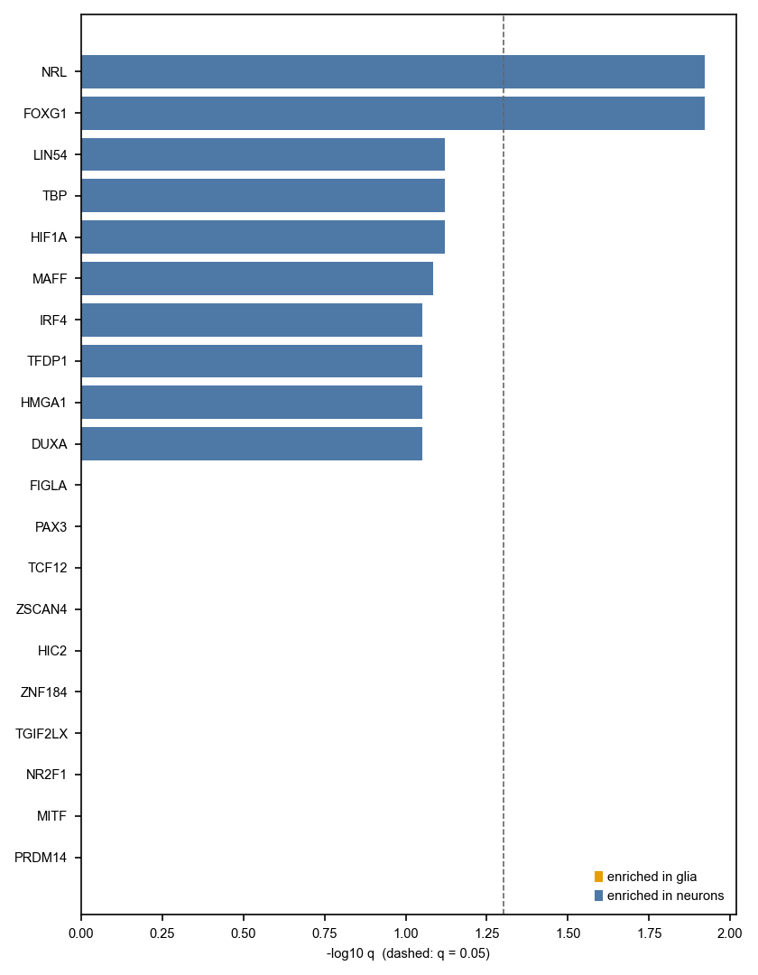
FOXG1, q = 0.012. FOXG1 is the forebrain neuronal transcription factor: it specifies telencephalic identity, and this is human middle temporal gyrus.
DLX2, the GABAergic factor, sits just below the line at q = 0.089. Both are
mechanistically right, and both survived the control that killed SOX9.
The reverse contrast, glia over neurons, gives nothing at q<0.05; MITF
and NR2F1 lead at q = 1.
10. Why there is no one-call version of this
Sections 8 and 9 do this by hand because the lesson is in the assembly. The obvious next step is a function that runs it per cell type — markers, their promoters, the scan, a test — and cytorete carried one during development. It was removed before release, because it was measured and it does not work. The measurement is more useful than the function, so here it is.
The question is real: which TF motifs sit in the promoters of what a cell type is specific for? It is cheap, it needs no ATAC, and everyone wants the answer. Two honest implementations were tried on SEA-AD MTG (24 subclasses, 19,271 genes with promoters, median promoter GC 0.54).
Attempt one: a Fisher test on the top markers
COSG markers per cell type, their promoters, one Fisher test per TF against a GC- and length-matched background — the control that §8’s SOX9 result failed. Motifs pooled per TF, so a well-catalogued family cannot outvote a sparse one.
| markers per cell type | significant TF × cell-type pairs at FDR < 0.05 |
|---|---|
| 50 | 0 |
| 100 | 1 (THAP1 in Microglia-PVM, OR 2.8) |
| 200 | 5 (THAP1 and SPIC in Microglia, NHLH1 in Pvalb, NKX6-3 in Sncg, RFX6 in L4 IT) |
The overlap between cutoffs is Jaccard 0.00 between 50 and 100, and 0.20 between 100 and 200. Any one of those runs, reported alone, would produce a short list that looks publishable, and the run beside it does not support it.
Drop the matched background and the same call returns ten significant pairs — GSX2, HOXA6, HOXB1, HOXB6, HOXB7, LHX5, MEOX2 — an AT-rich homeobox block, each in one cell type. Marker promoters are compositionally unlike the average promoter, and an unmatched test reports that composition as if it were regulation. That is §8’s lesson with a different family in the answer.
Attempt two: no cutoff at all, and PIASO’s own null
The cutoff instability suggests the cutoff is the flaw, so the second attempt
removes it. Each TF’s cistrome — every gene whose promoter carries its motif —
becomes a gene set, scored per cell with piaso.tl.score against size- and
expression-matched control sets, then ranked across cell types with COSG λ.
No top_n, and the same matched-control machinery regulonActivity and
SCALAR use.
| gene set per TF | sets | median size | own-TF agreement¹ | |
|---|---|---|---|---|
| whole promoter universe | every gene whose promoter carries the motif | 710 | 1,062 | 2.8 % |
| marker universe | the same, restricted to any type’s top-200 COSG markers | 693 | 130 | 4.0 % |
¹ TFs whose motif set is top-20 specific in the subclass where their own
expression is most specific. The same measurement on inferRegulon’s 415
regulons, same cells, same JASPAR motifs, is 26.7 % — seven to nine times
either row above.
CUX2’s motif set lands in OPC, RORB’s in astrocytes, FOXP2’s in VLMC. What does come out is family-level and only where a family happens to be lineage-restricted: ETS (SPIC, SPI1, ELF1/3, ETV6) in microglia, NR4A1/2 in astrocytes, CREB3 and XBP1 in oligodendrocytes.
Why no third attempt will fix it
A PWM is a family address, not a TF address. The sixty-odd ETS matrices in JASPAR pick nearly the same promoters; so do the homeobox block and the bHLH E-boxes. A gene set defined by the motif alone therefore carries no cell-type identity unless the family itself is lineage-restricted — which is exactly the three cases that light up above.
The only thing that separates SPI1 from ELF1, or CUX2 from every other
homeobox, is the TF’s own expression profile. Requiring the targets’
specificity to agree with the TF’s is not an optional refinement on top of a
motif test; it is the step that makes the answer about a TF at all. In cytorete
that step is cospecificity_trans, and the function that runs it is
inferRegulon.
So the one-call version of this section is
cytorete.tl.inferRegulon: the same promoters
and the same scan you built here, inside a model that also requires the TF and
its targets to be specific to the same cells. On this dataset that gives 412
regulons whose top hits are the factors the field would name.
If you want the raw matrix anyway — to test a gene list of your own, or to ask
a question this page has not — cytorete.pp.build_cistrome returns the sparse
TF × gene hit matrix and scipy.stats.fisher_exact is two lines away. What is
gone is the claim that running that test per cell type answers the question.
Regulatory regions beyond promoters
piaso.data also carries the SCREEN cCRE registry, so the same scan can run on
candidate enhancers instead:
ccres = piaso.data.load_screen_ccres(piaso.data.fetch_screen("hg38"), classes=("PLS", "pELS", "dELS"))sum(len(v["starts"]) for v in ccres.values())row = promoters(["SOX9"]).iloc[0]near = piaso.data.ccres_near_tss(ccres, row.chrom, int(row.start + UP), 100_000)len(near)Feed their sequences to extract_sequences and scan_motifs exactly as above, and match the background on GC, which matters more for enhancers than for
promoters, not less.