
GDR and SVD on 1.5 million cells
Two embeddings, one dataset, the same normalised layer underneath: the question this page answers is what each one costs and what you get for it, measured rather than asserted.
The dataset is a 1,501,089-cell human prefrontal cortex snMultiome atlas spanning the lifespan — 38,606 genes, 357 samples in 10 sequencing batches, 24 GB as a cytome. Every number below comes from one run on a 20-core workstation with 251 GB of RAM, of which the pipeline used at most 24.
import piaso
ds = piaso.data.load_dataset("humanlifespan_pfc_rna", return_type="cytome")path = ds.path          # every call below takes the file, and opens it itselfds.close()
return_type="cytome" downloads the file once and hands back an open dataset
rather than reading it into memory. At 24 GB that distinction is the whole
point.
One normalisation, two paths
Both paths read the same infog layer, so what is being compared is the
embedding and not a preprocessing choice.
piaso.tl.infog(path, n_top_genes=3000, save_layer=True)The SVD path is the conventional one:
piaso.tl.runSVD(path, layer="infog", n_components=50, key_added="X_svd")piaso.tl.neighbors(path, use_rep="X_svd", n_neighbors=15, key_added="svd")piaso.tl.umap(path, use_rep="X_svd", key_added="X_umap_svd", neighbors_key="svd")The GDR path embeds each batch on its own marker genes:
piaso.tl.runGDR(path, batch_key="batch", groupby=None, n_gene=20, layer="infog", key_added="X_gdr", max_workers=8)piaso.tl.neighbors(path, use_rep="X_gdr", n_neighbors=15, key_added="gdr")piaso.tl.umap(path, use_rep="X_gdr", key_added="X_umap_gdr", neighbors_key="gdr")groupby=None means GDR clusters within each batch rather than being handed
labels, so nothing about the known annotation enters either embedding. Both are
unsupervised; the labels below are only used to score the result afterwards.
What it costs
| step | time | peak RSS |
|---|---|---|
| INFOG normalisation | 27.4 min | 1.21 GB |
| SVD, 50 components | 19.3 min | 4.49 GB |
| neighbours + UMAP (SVD) | 44.1 min | 17.84 GB |
runGDR, 8 workers | 24.7 min | 10.51 GB |
| neighbours + UMAP (GDR) | 46.9 min | 23.67 GB |
| silhouette, 50,000 cells × 2 | 1.0 min | 7.72 GB |
| figures | 0.2 min | 5.35 GB |
| total | 163.6 min | 23.67 GB |
Two things are worth reading off that table.
The embeddings are the cheap part. GDR takes 24.7 minutes and SVD 19.3 — a five-minute difference on a dataset of this size. Between them the two neighbours-and-UMAP steps take 91 minutes, more than half the run, and they set the memory high-water mark. Choosing between GDR and SVD on runtime grounds is optimising the small term.
Memory is set by the graph, not by the matrix. INFOG streams the whole 1.5-million-cell matrix in 1.21 GB. The peak of 23.67 GB arrives during UMAP, which holds a k-nearest-neighbour graph in memory. Held dense, this matrix would be 1,501,089 × 38,606 × 4 bytes ≈ 232 GB before any analysis began.
What each embedding looks like
import matplotlib.pyplot as plt
piaso.settings.set_figure_params(style="cell")
# Both panels in one figure, on shared terms. Saved as two files, a difference# in point size or axis range between them reads as a difference in the data;# `piaso.pl.embedding` takes an `ax`, so it need not be.fig, axs = plt.subplots(1, 2, figsize=(13, 5.5))piaso.pl.embedding(path, basis="X_umap_svd", color="cell_type",                   ax=axs[0], show=False, title="SVD (50 dims)")piaso.pl.embedding(path, basis="X_umap_gdr", color="cell_type",                   ax=axs[1], show=False, title="GDR (315 dims)")fig.tight_layout()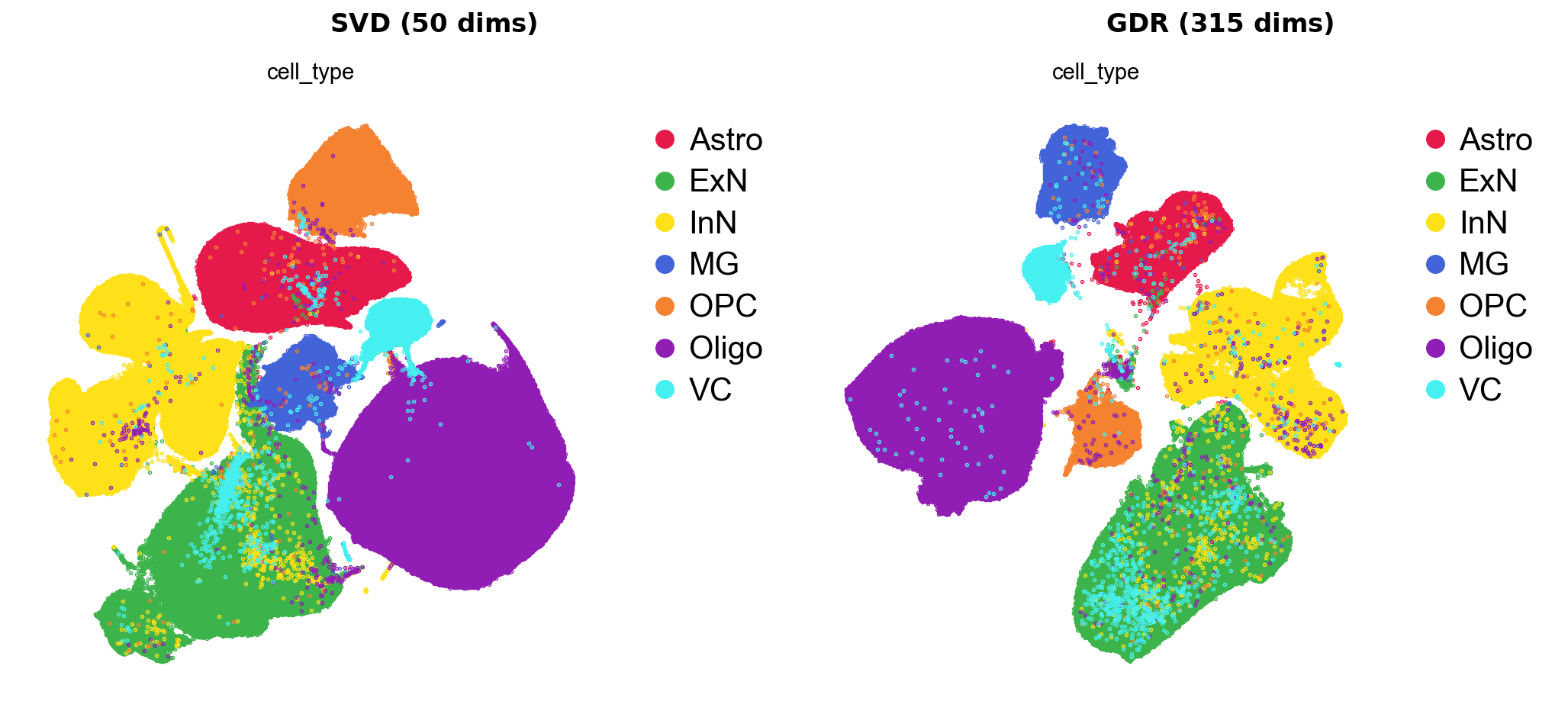
Both resolve the seven classes into contiguous territories, and neither shows donor or batch islands — with 357 samples across 10 batches, that is the first thing to check and the easiest to fail.
The difference is in the shape. GDR draws seven islands with visible space between them; SVD draws one connected mass with the classes as regions of it, excitatory and inhibitory neurons meeting along a shared border. That is the expected consequence of what GDR optimises: an axis per marker set makes between-type distances large relative to within-type ones.
At finer resolution the same distinction holds:
fig, axs = plt.subplots(1, 2, figsize=(13, 5.5))for ax, basis, title in ((axs[0], "X_umap_svd", "SVD (50 dims)"), (axs[1], "X_umap_gdr", "GDR (315 dims)")): piaso.pl.embedding(path, basis=basis, color="Subclass_predicted", ax=ax, show=False, title=title)fig.tight_layout()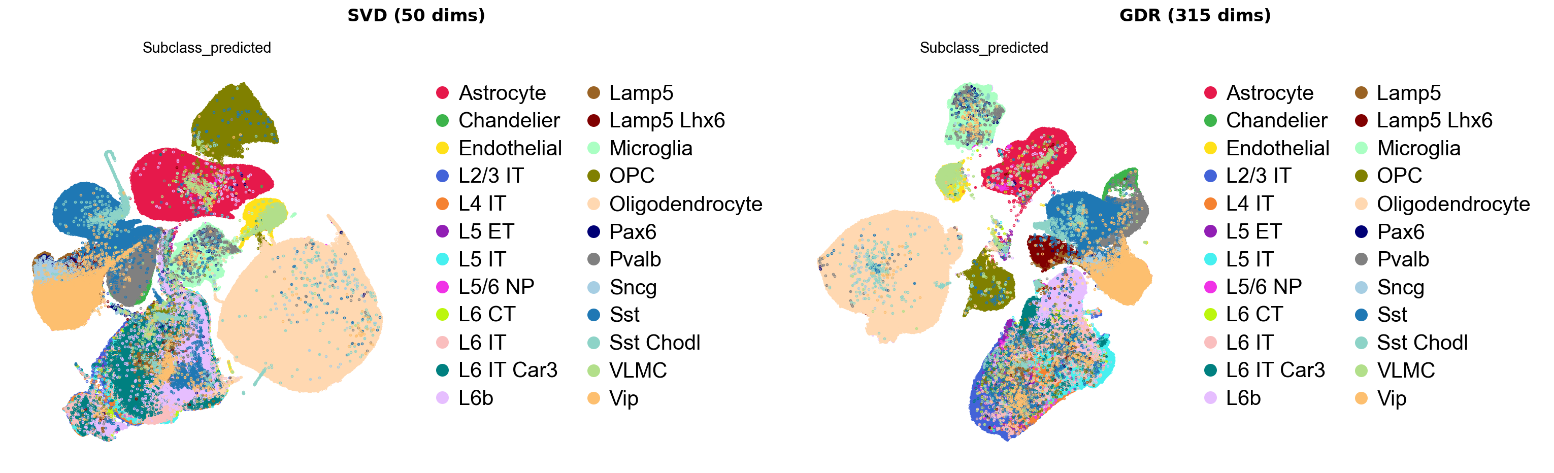
The 24 subclasses land inside the class territories rather than across them. The IT layers stay adjacent and partly overlapping in both — L2/3, L4, L5 and L6 IT are a gradient in the tissue, and an embedding that separated them cleanly would be worth distrusting.
Which one separates cell types better
The obvious measure is misleading, so it is worth doing carefully. Silhouette on the two embeddings as stored:
| dimensions | silhouette | |
|---|---|---|
| SVD | 50 | 0.512 |
| GDR | 315 | 0.321 |
Read at face value that says SVD wins by a wide margin. It does not. Euclidean distances concentrate as dimension grows: in 315 dimensions the gap between the nearest and furthest point in a cluster shrinks relative to its typical distance, and silhouette falls for reasons that have nothing to do with whether the cell types are separated. The two numbers are not measuring the same thing.
Two comparisons that are like-for-like — the first because it is rank-based and local, the second because both sides have the same dimensionality. Measured against the seven cell classes:
cell_type, 7 classes | kNN purity (k=15) | silhouette in 2-D UMAP |
|---|---|---|
| SVD | 0.9965 | 0.4405 |
| GDR | 0.9957 | 0.4683 |
On that labelling they are equivalent. Of a cell’s fifteen nearest neighbours, 99.6% carry its own label in both — a difference of eight cells in ten thousand, which is not a difference.
Stopping there would have been the wrong conclusion, because seven classes is an easy question. Oligodendrocytes and neurons separate in almost any embedding. The 24 predicted subclasses are the resolution the figures above are drawn at, and the resolution most analyses actually work at:
Subclass_predicted, 24 classes | kNN purity (k=15) | silhouette in 2-D UMAP |
|---|---|---|
| SVD | 0.8768 | 0.2543 |
| GDR | 0.9563 | 0.4440 |
Here they are not equivalent. GDR puts 95.6% of a cell’s neighbours in its own subclass against SVD’s 87.7% — 4.4% of neighbours misplaced rather than 12.3%, an error rate 2.8 times lower — and separates the subclasses in two dimensions nearly twice as well.
That is visible in the figures once you know to look: Chandelier, Lamp5 Lhx6, Pax6 and VLMC are their own islands in the GDR panel and are absorbed into the neighbouring interneuron mass in the SVD one.
The pattern is the one GDR is built for. SVD keeps the directions of greatest variance, and at 1.5 million cells the greatest variance is the difference between broad classes; rare subclasses contribute little of it and are not guaranteed an axis. GDR spends a dimension per marker set per batch, so a subclass that is 0.3% of the data gets the same representation as one that is 40%.
So the summary is not that they tie, and not that GDR is uniformly better:
- They agree on coarse structure. If seven classes is the question, SVD answers it as well as GDR, in 50 dimensions instead of 315 and five minutes less.
- They diverge on fine structure, and by enough to matter — 2.8× fewer misplaced neighbours at subclass resolution.
- GDR’s axes mean something. Its 315 dimensions are scores against marker gene sets, so a coordinate reads back as how strongly this cell expresses this batch’s markers for this cluster. An SVD component is a direction of variance and has no such reading.
Both stream from disk and neither needs the matrix in memory, which at 1.5 million cells is the constraint that decides whether the analysis runs at all.
Reproducing this
Everything on this page is in benchmarks/pfc_1p5m/:
run_gdr_vs_svd.py— the two pipelines, the timings and the memory figures, written tometrics.json;make_comparison_figure.py— the two-panel UMAPs;fair_compare.py— the kNN purity and 2-D silhouette numbers, written tofair_compare.json.
The memory sampler walks the process tree every half second, so the peaks include the GDR workers rather than only the parent.
Timings are one run on one machine. The memory figures are the stable part — they are set by chunk size and worker count, not by dataset size — and the runtimes will move with core count and disk.