Parse Evercode v4 (84k human PBMCs across two donors)
Combinatorial split-pool barcoding (Parse Biosciences Evercode WT v4) differs from droplet scRNA-seq in two ways that matter immediately when you open the files:
- The raw matrix is already cells × genes, and it includes the ambient tail.
split-pipewritesDGE.mtx.gzwith barcodes as rows (cell_metadata.csv.gz) and genes as columns (all_genes.csv.gz), down to 10 transcripts per barcode combination. Across these two PBMC donors that is 672,628 barcode combinations with a median of 13 UMIs. Filtering out the ambient wells (min_counts=500, min_features=300) comes before QC violins and doublet simulation, not after. - Per-cell read and transcript counts sit right in
cell_metadata.csv.gz. Becausemread_count(mapped reads) andtscp_count(unique transcripts / UMIs) are recorded for every cell, per-cell sequencing saturation and reads-per-UMI can be inspected alongside standard gene and mitochondrial metrics.
This tutorial takes two Parse Evercode WT v4 human PBMC donor libraries (86,973 cell-called barcodes → 82,031 high-quality cells across 62,710 genes) from the public Parse Biosciences dataset (Performance of Evercode WT v4 in Human Immune Cells (PBMCs)) through sequencing QC, per-donor Scrublet doublet removal, INFOG normalization, SVD vs GDR donor integration (batch_key="donor"), dual annotation with KAMON and PIASOmarkerDB, and COSG marker discovery.
from pathlib import Pathimport anndata as adimport cosgimport matplotlib.pyplot as pltimport numpy as npimport pandas as pdimport piasoimport scipy.ioimport scipy.sparse as spfrom sklearn.metrics import silhouette_score
piaso.settings.set_figure_params(style="cell")
1. Load the Parse split-pipe donor outputs
The raw split-pipe output directories (Parse_Evercode_v4-PBMC_Donor1 and Parse_Evercode_v4-PBMC_Donor2) are available from Parse Biosciences at https://www.parsebiosciences.com/datasets/performance-of-evercode-wt-v4-in-human-immune-cells-pbmcs/. Each donor folder contains three gzipped files:
DGE.mtx.gz— MatrixMarket sparse count matrix (cells × genes)cell_metadata.csv.gz— barcode well coordinates (bc1_well,bc2_well,bc3_well) and per-barcode read/transcript totals (mread_count,tscp_count,gene_count)all_genes.csv.gz— Ensemblgene_id,gene_name, andgenome
def load_parse_donor(donor_dir: str | Path, donor_label: str) -> ad.AnnData:    donor_dir = Path(donor_dir)    obs = pd.read_csv(donor_dir / "cell_metadata.csv.gz", index_col=0)    var = pd.read_csv(donor_dir / "all_genes.csv.gz")
    gene_names = var["gene_name"].fillna(var["gene_id"]).astype(str).to_numpy()    var.index = pd.Index(gene_names, name="gene_name")
    X = scipy.io.mmread(str(donor_dir / "DGE.mtx.gz"))    if X.shape[0] == len(obs) and X.shape[1] == len(var):        X = sp.csr_matrix(X, dtype=np.float32)    else:        X = sp.csr_matrix(X.T, dtype=np.float32)
    adata = ad.AnnData(X=X, obs=obs, var=var)    adata.var_names_make_unique()    adata.obs_names = [f"{donor_label}_{bc}" for bc in adata.obs_names]    adata.obs["donor"] = donor_label    return adata

data_root = Path("ParseBio_PBMC_evercodeV4")ad1 = load_parse_donor(data_root / "Parse_Evercode_v4-PBMC_Donor1", "Donor1")ad2 = load_parse_donor(data_root / "Parse_Evercode_v4-PBMC_Donor2", "Donor2")adata_raw = ad.concat([ad1, ad2], join="inner", merge="same")del ad1, ad2adata_raw.shape
(672628, 62710)Separate real cells from the split-pool ambient tail
In Parse split-pipe outputs, DGE.mtx.gz retains every barcode combination with at least 10 transcripts (285,116 barcodes in Donor 1 and 387,512 in Donor 2; median 13 transcripts). Running doublet simulation on 672,628 mostly empty barcode combinations would pair ambient wells with each other. Apply the lower-bound cell-calling filter (min_counts=500, min_features=300) first:
adata = adata_raw.copy()piaso.pp.filter_cells(adata, min_counts=500, min_features=300)del adata_rawadata.obs["donor"].value_counts()donorDonor2 44921Donor1 42052Name: count, dtype: int64That retains 86,973 cells (42,052 from Donor 1 and 44,921 from Donor 2).
2. Sequencing and quality-control metrics
piaso.pp.calculateCellMetrics computes n_counts, n_genes, pct_counts_mt, and pct_counts_ribo in a single pass. Because Parse records mread_count (mapped reads per cell) and tscp_count (UMIs per cell) in adata.obs, we also compute reads per UMI (mread_count / tscp_count) and per-cell sequencing saturation (100 × (1 - tscp_count / mread_count)):
piaso.pp.calculateCellMetrics(    adata,    prefix_vars={"mt": "MT-", "ribo": ["RPS", "RPL"]},)
adata.obs["reads_per_umi"] = ( adata.obs["mread_count"] / np.maximum(adata.obs["tscp_count"], 1)).astype(np.float32)adata.obs["sequencing_saturation"] = ( (1.0 - adata.obs["tscp_count"] / np.maximum(adata.obs["mread_count"], 1)) * 100.0).astype(np.float32)| Donor | Cells (≥ 500 UMIs, ≥ 300 genes) | Median UMIs (n_counts) | Median genes (n_genes) | Median mapped reads (mread_count) | Median reads / UMI | Median saturation (%) | Median %MT | Median %Ribo |
|---|---|---|---|---|---|---|---|---|
| Donor1 | 42,052 | 9,959 | 3,172 | 22,220 | 2.23 | 55.2% | 2.13% | 0.94% |
| Donor2 | 44,921 | 10,604 | 3,380 | 23,711 | 2.24 | 55.3% | 2.69% | 0.74% |
Both donors are deeply sequenced (~10,000 UMIs and ~3,300 genes per cell at 55% saturation) with low mitochondrial fractions (2.13% and 2.69%). Notice also that whole-transcriptome random hexamer + oligo-dT priming in Evercode v4 yields a much lower ribosomal protein mRNA fraction (< 1%) than 3’ droplet PBMC libraries.
piaso.pl.plot_features_violin( adata, [ "n_genes", "n_counts", "pct_counts_mt", "pct_counts_ribo", "mread_count", "sequencing_saturation", ], groupby="donor", ncol=3, width_single=3.3, height_single=2.8,)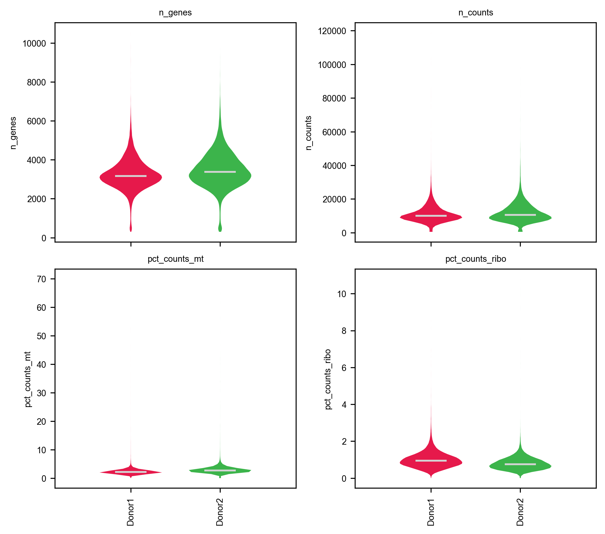
3. Per-donor doublet detection (Scrublet) and two-tailed QC
Doublets only form between cells processed within the same donor sample, so library_key="donor" runs Scrublet independently inside Donor1 and Donor2:
piaso.pp.scrublet(    adata,    library_key="donor",    expected_doublet_rate=0.04,    random_state=0,)
adata.obs.groupby("donor", observed=True).agg( called_doublets=("is_doublet", "sum"), n_cells=("is_doublet", "size"), doublet_pct=("is_doublet", lambda s: round(100.0 * s.mean(), 2)), median_score=("scrublet_score", "median"),)| Donor | Cells | Called doublets | Doublet rate (%) | Median scrublet_score |
|---|---|---|---|---|
| Donor1 | 42,052 | 1,184 | 2.82% | 0.0171 |
| Donor2 | 44,921 | 1,716 | 3.82% | 0.0166 |
Inspect the joint distributions of UMIs, detected genes, mitochondrial percentage, and Scrublet scores before cutting:
fig, axes = plt.subplots(1, 2, figsize=(10.5, 4.2))for i, (donor_id, col) in enumerate([("Donor1", "#1f77b4"), ("Donor2", "#ff7f0e")]):    sub = adata.obs[adata.obs["donor"] == donor_id]    axes[0].scatter(        sub["n_counts"], sub["n_genes"],        s=1.5, alpha=0.25, c=col, label=donor_id, rasterized=True,    )axes[0].axhline(300, color="crimson", ls="--", lw=1)axes[0].axvline(29150, color="crimson", ls="--", lw=1)axes[0].set_xlabel("Total UMIs (n_counts)")axes[0].set_ylabel("Detected genes (n_genes)")axes[0].set_title("UMIs vs Genes per Cell")axes[0].legend(frameon=False, markerscale=4)
sc = axes[1].scatter(    adata.obs["n_counts"],    adata.obs["pct_counts_mt"],    c=adata.obs["scrublet_score"],    s=1.5, alpha=0.35, cmap="viridis", vmin=0, vmax=0.4, rasterized=True,)axes[1].axhline(5.2, color="crimson", ls="--", lw=1)axes[1].axvline(29150, color="crimson", ls="--", lw=1)axes[1].set_xlabel("Total UMIs (n_counts)")axes[1].set_ylabel("Mitochondrial reads (%)")axes[1].set_title("UMIs vs %MT (colored by Scrublet score)")plt.colorbar(sc, ax=axes[1], label="Scrublet score")plt.tight_layout()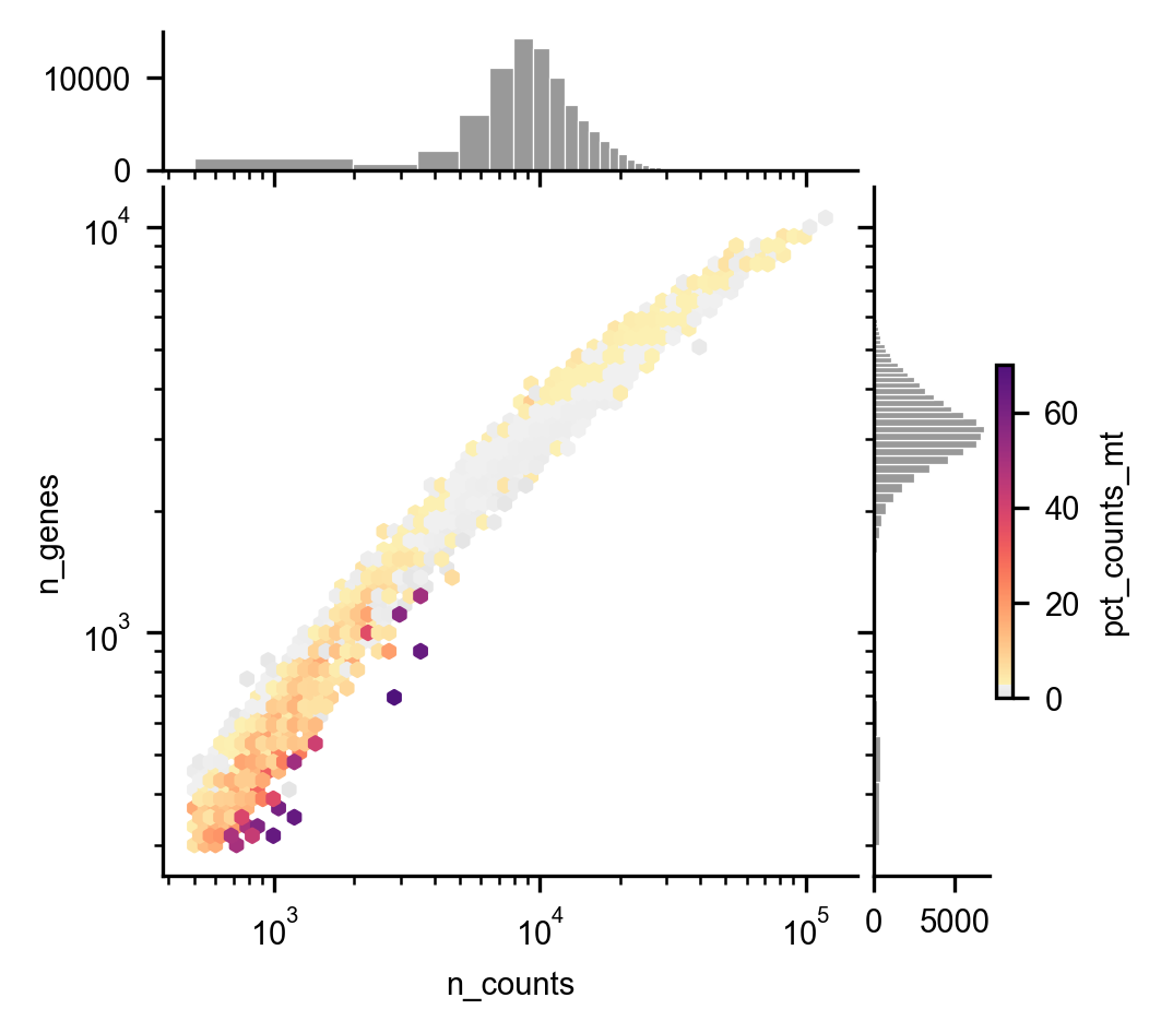
Remove doublets (is_doublet or scrublet_score > 0.25), upper-tail UMI outliers (max_counts=29150, 99th percentile), and damaged cells with elevated mitochondrial reads (max_pct_mt=5.2%, 98th percentile):
keep = ( (~adata.obs["is_doublet"].astype(bool)) & (adata.obs["scrublet_score"] <= 0.25) & (adata.obs["pct_counts_mt"] <= 5.2) & (adata.obs["n_counts"] <= 29150))adata = adata[keep].copy()adata.shape(82031, 62710)86,973 → 82,031 cells (40,288 from Donor 1 and 41,743 from Donor 2).
4. INFOG normalization and baseline SVD embedding
Preserve the raw UMI counts in adata.layers["counts"], normalize and select the top 3,000 informative genes with piaso.tl.infog, and compute a 50-component SVD baseline:
adata.layers["counts"] = adata.X.copy()
piaso.tl.infog(adata, layer="counts", n_top_genes=3000)piaso.tl.runSVD(adata, layer="infog", use_highly_variable=True, n_components=50, key_added="X_svd")piaso.tl.neighbors(adata, use_rep="X_svd", n_neighbors=15, random_state=42, key_added="neighbors_svd")piaso.tl.leiden(adata, resolution=1.0, neighbors_key="neighbors_svd", key_added="leiden_svd")piaso.tl.umap(adata, neighbors_key="neighbors_svd", key_added="X_umap_svd")
piaso.pl.embedding(    adata,    basis="X_umap_svd",    color=["donor", "leiden_svd"],    legend_loc=["right margin", "on data"],    ncol=2,)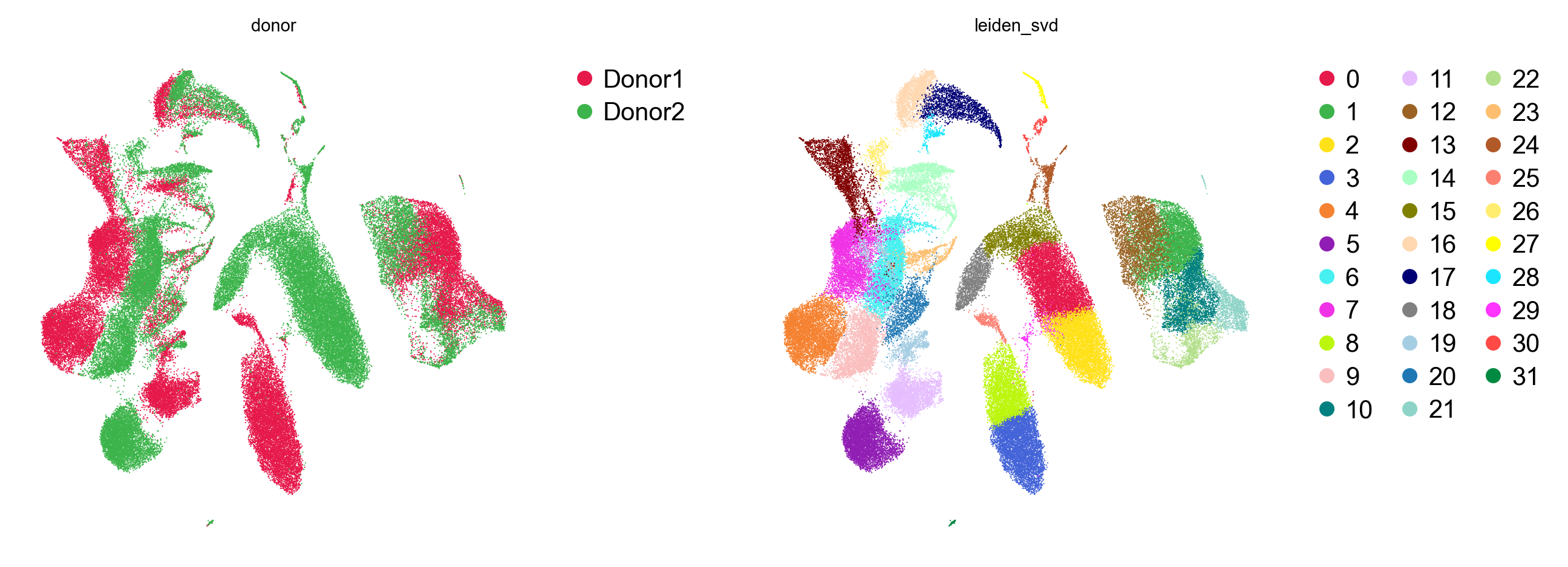
In the unintegrated SVD embedding (32 clusters), donor-specific shifts remain visible inside the monocyte and naive T-cell compartments (donor silhouette score 0.0402).
5. Multi-donor integration with GDR (batch_key="donor")
Rather than warping principal components after the fact, piaso.tl.runGDR selects cell-identity marker gene sets within each donor (batch_key="donor") and embeds all 82,031 cells directly along shared biological identity axes:
piaso.tl.runGDR(    adata,    batch_key="donor",    groupby=None,    n_gene=30,    mu=10.0,    resolution=1.5,    layer="infog",    infog_layer="counts",    score_layer="infog",    key_added="X_gdr",    max_workers=8,)
piaso.tl.neighbors(adata, use_rep="X_gdr", n_neighbors=15, random_state=42, key_added="neighbors_gdr")piaso.tl.leiden(adata, resolution=1.0, neighbors_key="neighbors_gdr", key_added="leiden")piaso.tl.umap(adata, neighbors_key="neighbors_gdr", key_added="X_umap")
piaso.pl.embedding(    adata,    basis="X_umap",    color=["donor", "leiden"],    legend_loc=["right margin", "on data"],    ncol=2,)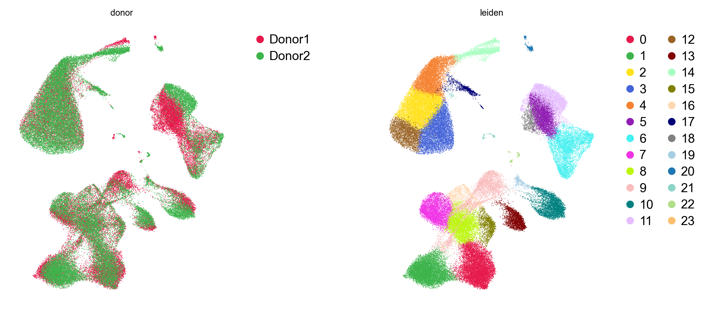
Measuring SVD vs GDR
Compare the two embeddings on the same 82,031 cells using the silhouette score of the donor label (lower = better donor mixing) and the cell-type label (higher = better biological separation):
sil_svd_donor = silhouette_score(adata.obsm["X_svd"], adata.obs["donor"], sample_size=10000, random_state=42)sil_gdr_donor = silhouette_score(adata.obsm["X_gdr"], adata.obs["donor"], sample_size=10000, random_state=42)| Embedding | Runtime (82,031 cells) | Clusters (res=1.0) | Donor silhouette (lower is better) | Cell-type silhouette (higher is better) |
|---|---|---|---|---|
SVD (X_svd) | 113.9 s | 32 | 0.0402 | 0.2017 |
GDR (X_gdr, batch_key="donor") | 102.7 s | 24 | 0.0090 (4.5× lower) | 0.2237 (+11%) |
runGDR reduces donor separation 4.5× (0.0402 → 0.0090) while sharpening immune cell-type boundaries (0.2017 → 0.2237) and consolidating donor-split clusters from 32 down to 24.
6. Cell-type annotation with KAMON and PIASOmarkerDB
PIASO provides two complementary ways to annotate cell types using PIASOmarkerDB:
- Single-cell graph-smoothed annotation (
piaso.tl.kamon) — scores every cell against a reference marker study (AllenHumanImmuneHealthAtlas_L2) and diffuses those scores over the GDR kNN graph (neighbors_gdr). - Cluster-level de novo marker matching (
piaso.tl.analyzeMarkers) — runs COSG on the unsupervised Leiden clusters and queries the top markers against all 36 studies in PIASOmarkerDB.
Single-cell annotation with KAMON
piaso.tl.kamon( adata, study="AllenHumanImmuneHealthAtlas_L2", score_layer="infog", use_rep="X_gdr", neighbors_key="neighbors_gdr", key_added="cell_type",)adata.obs["cell_type"].value_counts().head(15)cell_typeCD14 monocyte 19001Naive CD4 T cell 12230Naive B cell 9458Memory CD4 T cell 7970Naive CD8 T cell 7606Intermediate monocyte 4982CD56dim NK cell 3719Memory B cell 3400MAIT 2676Memory CD8 T cell 2351CD16 monocyte 2051Treg 1532Effector B cell 1108CD8aa 800cDC2 629Name: count, dtype: int64piaso.tl.kamon annotates all 82,031 cells in 14.8 s across 27 immune populations.
piaso.pl.embedding( adata, basis="X_umap", color="cell_type", legend_loc="right margin",)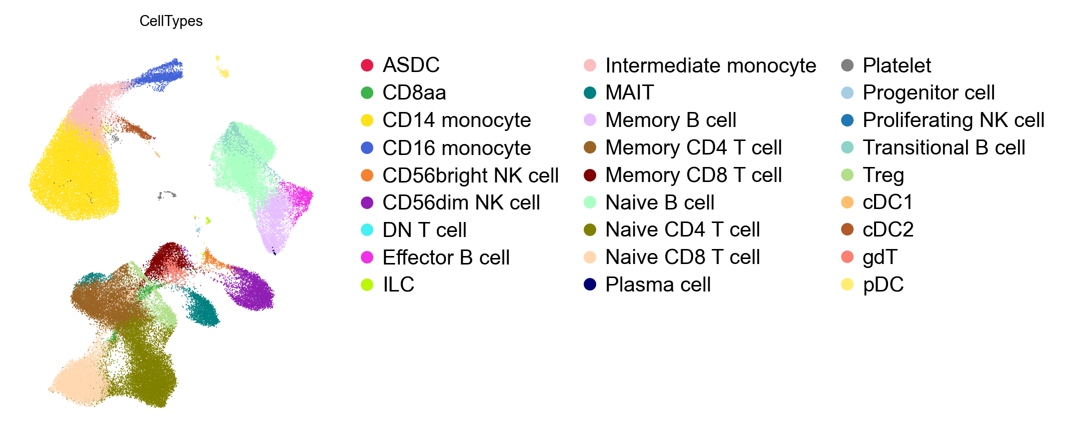
Splitting the embedding by donor confirms that every major and rare population (including cDC1, cDC2, pDC, CD56bright NK, Treg, MAIT, gdT, and Progenitor cell) is shared across both donors:
piaso.pl.plot_embeddings_split( adata, basis="X_umap", color="cell_type", splitby="donor",)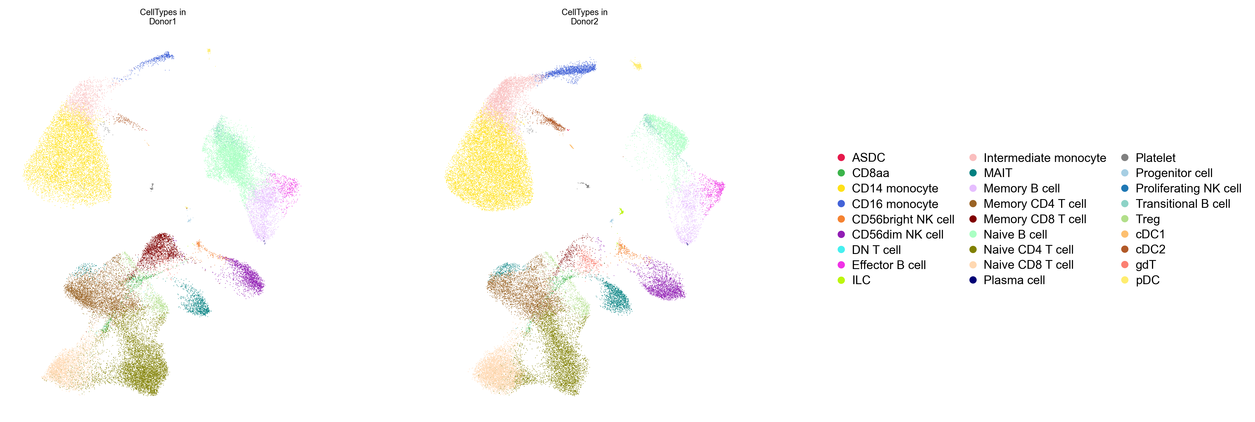
Cross-checking clusters against all 36 studies in PIASOmarkerDB
To cross-check the single-cell KAMON labels without restricting to a single reference study, run COSG on the 24 Leiden clusters and query PIASOmarkerDB with piaso.tl.analyzeMarkers:
cosg.cosg(    adata,    key_added="cosg_leiden",    groupby="leiden",    mu=100,    n_genes_user=50,    layer="infog",)
markerdb_res = piaso.tl.analyzeMarkers(adata.uns["cosg_leiden"])markerdb_res.predicted_cell_types| Leiden | Cells | Top 5 COSG markers | Top PIASOmarkerDB match | Reference study |
|---|---|---|---|---|
| 0 | 8,845 | FHIT, MIR99AHG, EDAR, ADTRP, SORCS3 | naive thymus-derived CD4+ αβ T cell | AsianImmuneDiversityAtlas2025 |
| 1 | 8,559 | NRCAM, LINC02446, PTPRK-AS1, ROBO1, FCGBP | naive thymus-derived CD8+ αβ T cell | AsianImmuneDiversityAtlas2025 |
| 2 | 8,382 | NRG1, LYZ, FCN1, S100A9, CD14 | Core CD14 monocyte | AllenHumanImmuneHealthAtlas2025_L3 |
| 3 | 6,313 | G0S2, AQP9, ACSL1, CXCL8, LUCAT1 | MONOCYTE_III_IL1B | SuoTeichmann2022_FetalImmune |
| 4 | 5,955 | SASH1, PID1, SH3PXD2B, TMEM51 | Intermediate monocyte | AllenHumanImmuneHealthAtlas2025_L2 |
| 5 | 5,378 | DSP, FCER2, LARGE1, SYN3, ADAM28 | naive B cell | XuTeichmann2023_BoneMarrow |
| 6 | 5,083 | COL4A3, COL4A4, TNFRSF13B, EML6 | memory B cell | AsianImmuneDiversityAtlas2025 |
| 7 | 4,692 | MTUS2, MYO16, GREM2, MB21D2, LINC00511 | effector memory CD4+ αβ T cell | XuTeichmann2023_LymphNode |
| 8 | 4,623 | ST8SIA1, TSHZ2, ICOS, SGPP2 | central memory CD4+ αβ T cell | AsianImmuneDiversityAtlas2025 |
| 9 | 4,490 | SGCD, KLRA1P, TRGC2, MYO6 | KLRF1+ GZMB+ CD27- EM CD8 T cell | AllenHumanImmuneHealthAtlas2025_L3 |
| 10 | 3,777 | BNC2, LINGO2, KLRF1, GRIK4 | CD56dim NK cell | AllenHumanImmuneHealthAtlas2025_L2 |
| 11 | 3,378 | RAPGEF5, PLD5, PCDH9 | B cell | EmontRosen2022_Adipose_Human_celltype |
| 12 | 3,021 | SERPINB2, PADI4, TDRD9, SPOCK1, BPI | CD14 monocyte | AllenHumanImmuneHealthAtlas2025_L2 |
| 13 | 2,213 | SLC4A10, ME1, IL23R, ADAM12 | mucosal invariant T cell (MAIT) | AsianImmuneDiversityAtlas2025 |
| 14 | 2,168 | UICLM, GPR20, RDUR | CD16 monocyte | AllenHumanImmuneHealthAtlas2025_L2 |
| 15 | 1,398 | RBMS3, LINC01281, RTKN2, FOXP3 | Treg | AllenHumanImmuneHealthAtlas2025_L2 |
| 16 | 946 | LINC02694, DUSP4, TSHR, LINC01362 | regulatory T cell | AsianImmuneDiversityAtlas2025 |
| 17 | 824 | ST18, DTNA, LRP1B, NCKAP5 | CD1c+ myeloid dendritic cell (cDC2) | AsianImmuneDiversityAtlas2025 |
| 18 | 755 | CCND1, ENPP1, CLNK, FCER2, LARGE1 | B cell | AsianImmuneDiversityAtlas2025 |
| 19 | 385 | SPTSSB, XCL1, TNFRSF11A, NFILZ | CD16- CD56bright NK cell | AsianImmuneDiversityAtlas2025 |
| 20 | 350 | LINC01478, CLEC4C, EPHB1, COL26A1 | plasmacytoid dendritic cell (pDC) | XuTeichmann2023_BoneMarrow |
| 21 | 217 | TUBB1, ITGB3, CAVIN2, SPARC, PF4 | Platelet | AllenHumanImmuneHealthAtlas2025_L3 |
| 22 | 207 | HDC, AKAP12, GCSAML, SLC24A3 | mast cell / basophil / ILC | XuTeichmann2023_Spleen |
| 23 | 72 | FANK1, COLEC12, VENTX, SLC46A2 | classical monocyte | XuTeichmann2023_Spleen |
The Sankey diagram (piaso.pl.sankey) and donor composition barplot (piaso.pl.stacked_barplot) show how the 24 unsupervised Leiden clusters map onto the KAMON immune cell types and how evenly the two donors contribute to each population:
piaso.pl.sankey( adata, left="leiden", right="cell_type", flow_scale="sqrt", title="Leiden clusters vs KAMON immune cell types",)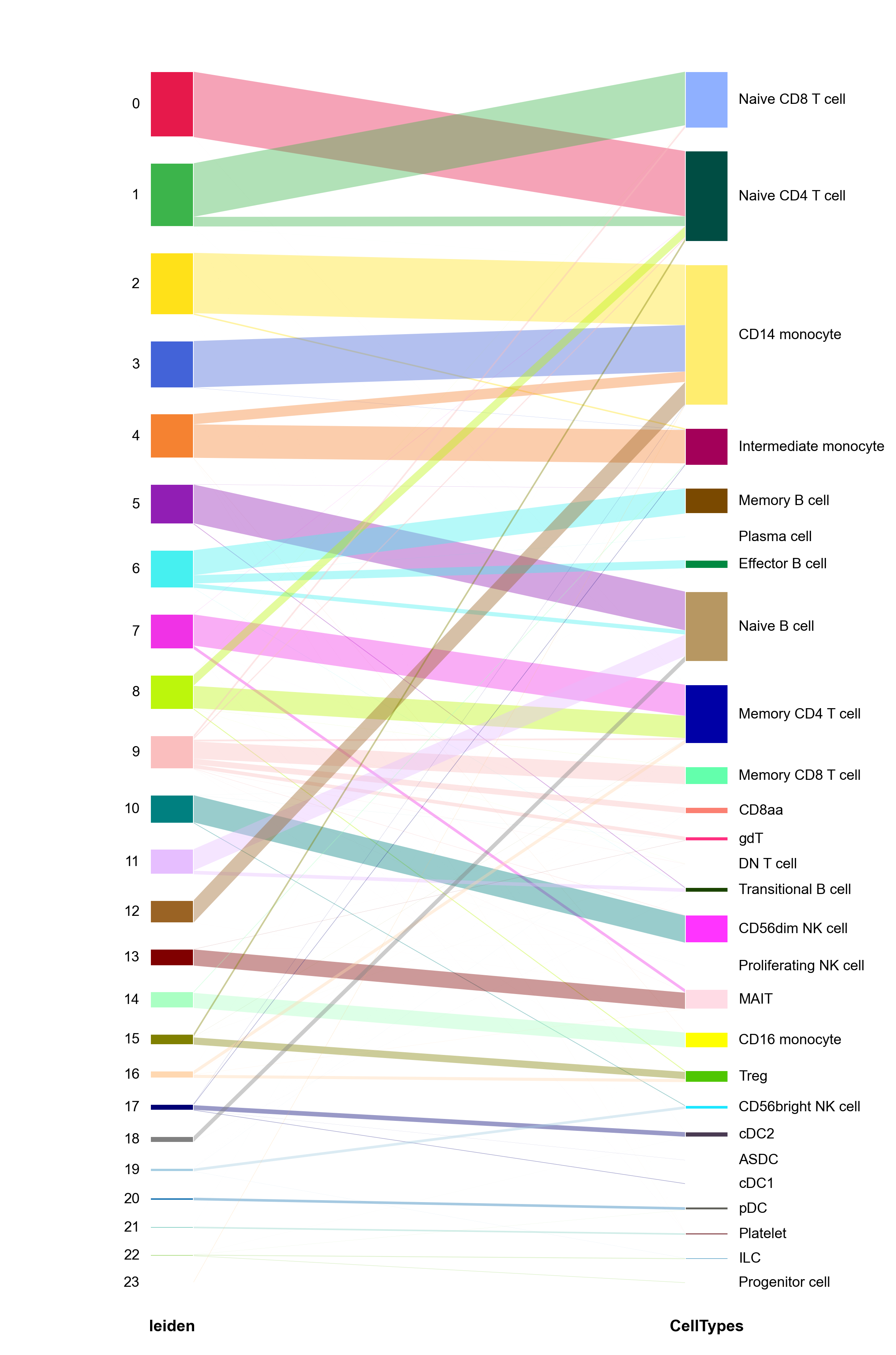
piaso.pl.stacked_barplot( adata, groupby="cell_type", color_by="donor", normalize=True, ylabel="Donor fraction", title="Donor composition across immune cell types",)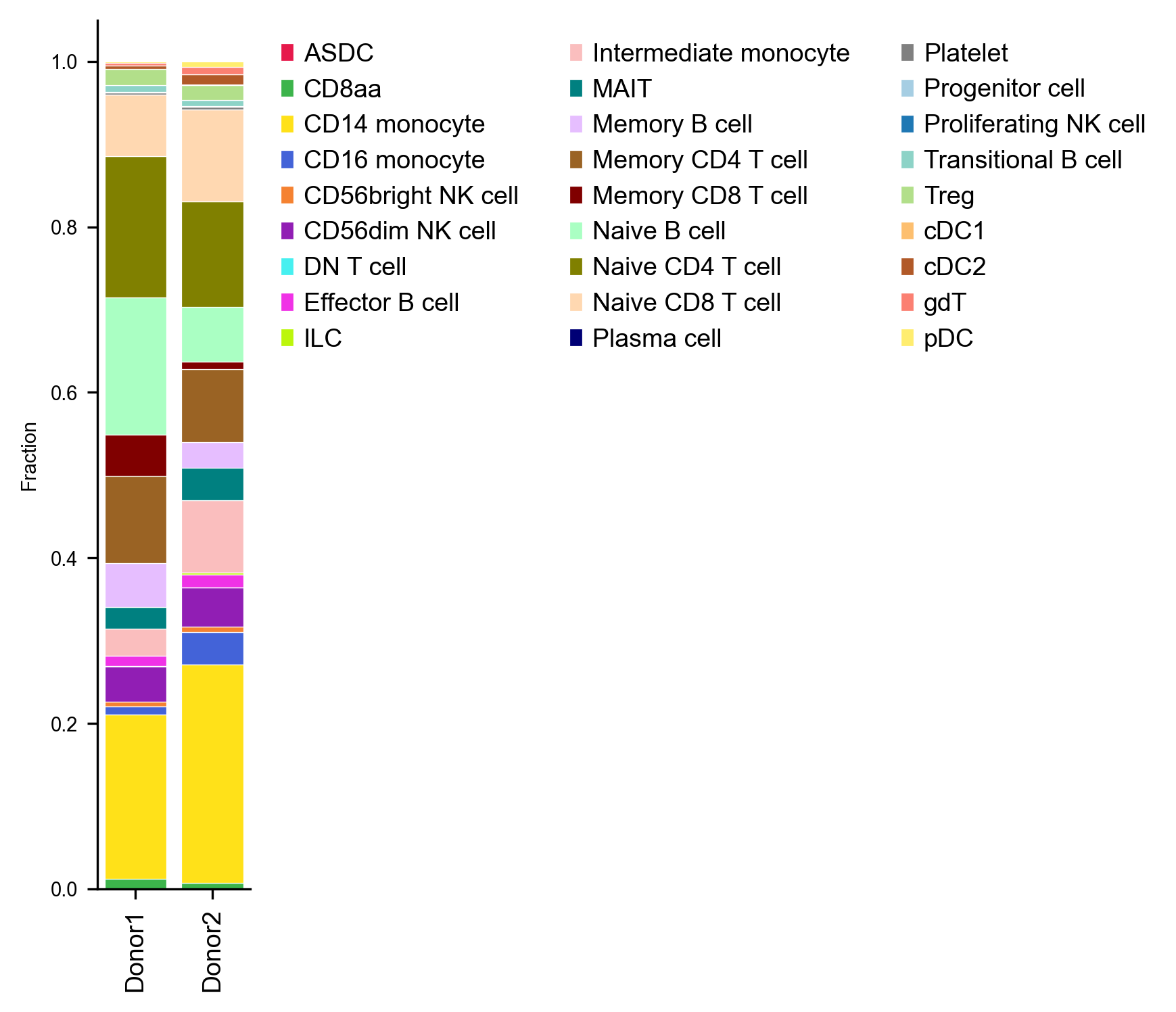
We can also inspect how transcript depth, mitochondrial fraction, and sequencing saturation vary by immune lineage (piaso.pl.plot_group_metrics) — monocytes and dendritic cells carry roughly twice the transcripts of resting lymphocytes:
piaso.pl.plot_group_metrics( adata, groupby="cell_type", metrics=["n_counts", "n_genes", "pct_counts_mt", "sequencing_saturation"],)
7. COSG marker gene discovery and plots
Finally, run COSG across the annotated immune cell types to identify specific marker genes for every population:
cosg.cosg( adata, key_added="cosg_celltype", groupby="cell_type", mu=100, n_genes_user=30, layer="infog",)Plot the top 3 COSG markers per immune cell type in a standardized dotplot:
names_df = pd.DataFrame(adata.uns["cosg_celltype"]["names"])top_markers, seen = [], set()for ct in adata.obs["cell_type"].value_counts().head(20).index:    if ct in names_df.columns:        for g in names_df[ct]:            if g in adata.var_names and not str(g).startswith("ENSG") and g not in seen:                top_markers.append(g)                seen.add(g)                if sum(1 for x in top_markers if x in set(names_df[ct][:8])) >= 3:                    break
piaso.pl.dotplot(    adata,    var_names=top_markers,    groupby="cell_type",    layer="infog",    standard_scale="var",)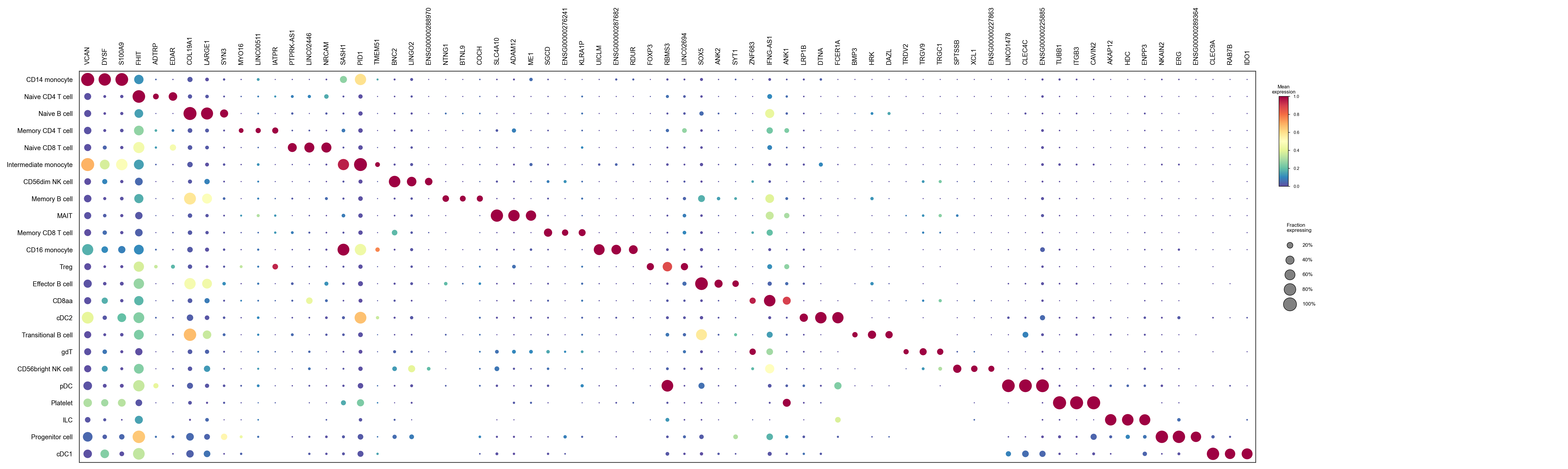
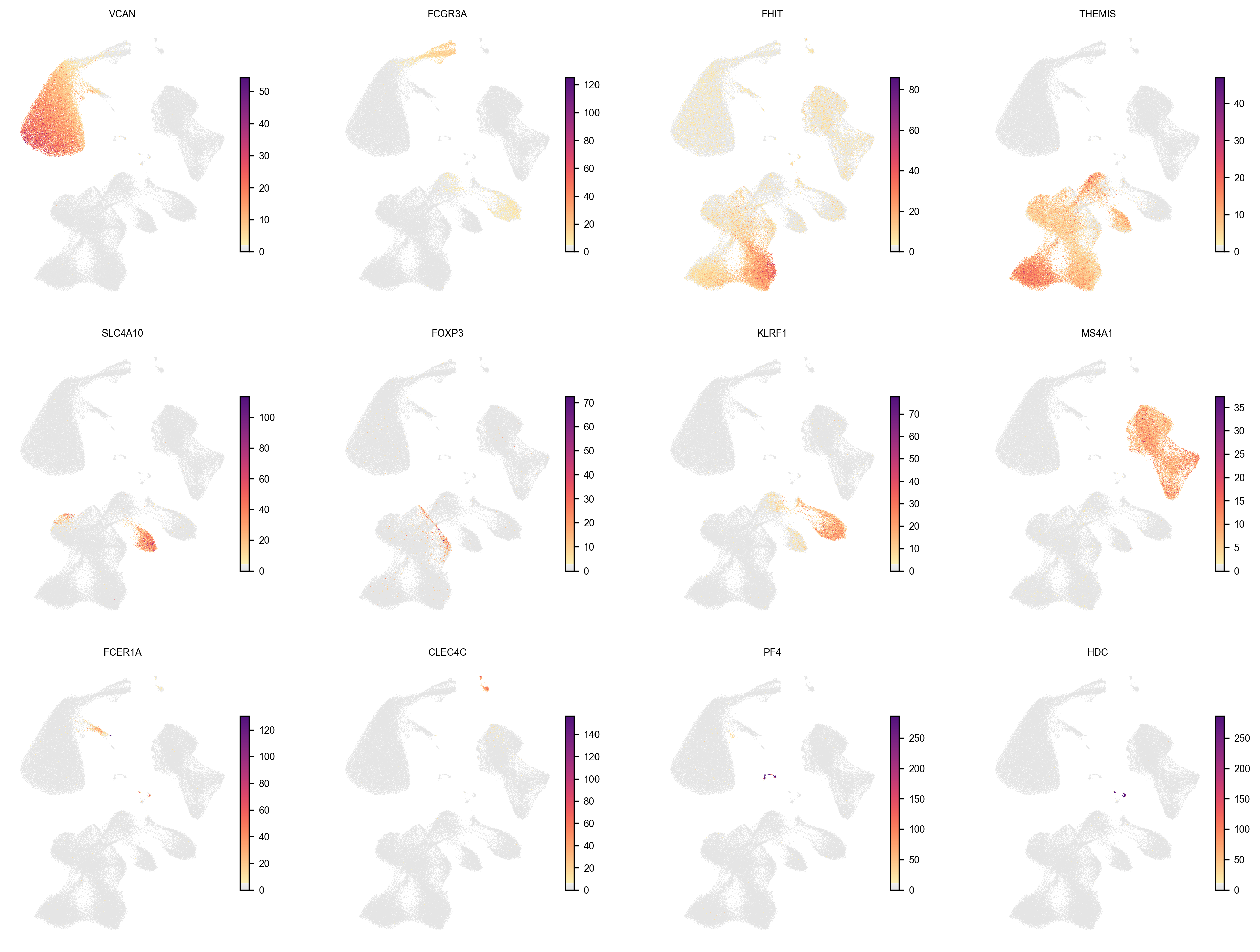
And visualize canonical and COSG-selected lineage markers directly on the GDR UMAP:
piaso.pl.embedding( adata, basis="X_umap", color=[ "VCAN", "FCGR3A", "FHIT", "THEMIS", "SLC4A10", "FOXP3", "KLRF1", "MS4A1", "FCER1A", "CLEC4C", "PF4", "HDC", ], layer="infog", cmap=piaso.pl.color.c_color1, ncol=4,)